install.packages(c("sf", "stars", "tidyverse", "tigris", "leaflet", "cowplot", "cartogram"))Setting The Stage
(Almost) All Data Is Spatial
When conducting population research, almost everything has a spatial aspect to it. We often may not have access to this spatial resolution, but for those data that we do, it is important to incorporate spatial techniques to explore our data.
Exploring our data through a spatial lense allows us to answer questions like:
- How does a variable vary by region?
- Is there a relationship between variables by region?
- How many facilities are within a region?
- How far is the nearest facility?
- Does proximity to a facility have a relationship with another variable?
- How has a variable changed over time?
Before you participate in this training, think about what questions you want to explore.
Looking To Learn More?
The following training was created with the intention to get you up to speed as quick as possible. It is very possible we left something out that may be important to you. For more extensive reading about geocomputation using R, we recommend Spatial Data Science and Geocomputation with R.
If you are looking to learn how to use the R and the tidyverse for data science, we recommend R for Data Science. For more information about how R the programming language works, we recommend Advanced R.
Packages
Since R is open source, anyone can make a package! It also means that there are lots of useful packages to pick from. The following are a non-exhaustive list of some the packages that we use most often. We encourage you to explore beyond this list. For this training, we will only be using these packages and their dependencies.
sf- The primary package for vector-based geospatial computation within R. One of the most useful aspects about sf is that it allows you to interact with the attribute tables of spatial objects in much the very same ways you would atibbleordata.table.stars- One of two main modern packages for raster-based geospatial data. Also offers the ability the work with multidimensional data. Made by the same people who made sf, and is therefore very well integrated.tidyverse- A collection of data science related packages that is fairly ubiquitious throughout R. It is developed by Posit who make RStudio.tigris- A package that allows users to download Census geometries using the Census API. Often, we rely on Census boundaries, so tigris makes getting that data easier and more repeatable.tidycensus- A package that allows users to download Census variables and tables using the Census API. Can be really useful for the tedious process of extracting census variables. In this training, we use it to make a dot density map.leaflet- An R interface for the Leaflet open-source JavaScript library that allows R users to easily construct interactive maps.cowplot- An add-on package toggplot2(from the tidyverse) that aids with making “publication-ready figures”. Its developer, Claus O. Wilke, has a great book on data visualization called Fundamentals of Data Visualization, where he uses cowplot extensively.cartogram- A package to create cartograms. Simple as that.
Use the following command to install the above packages.
File Formats
Shapefiles are the most ubiquitous geospatial vector format. They were developed by ESRI in the early 1990s and have aged since. Although they still widely used, they have several limitations
- Maximum size is 2 GB
- Maximum length of field names is 10 characters
- Maximum number of fields is 255
- No support for NULL values
They, counterintuitively, are made up of several files of which only three are mandatory.
- .shp – stores feature geometry
- .shx – stores the positional index of the feature geometry
- .dbf – stores the attribute table for the geometry
File geodatabases are a collection of a files in a folder that can store vector, raster, and even non-spatial data. A single file geodatabase can store over 2 billion features or tables. They are great for sharing data with collaborators who use ESRI products.
Field names are limited to 64 characters. The default maximum size of datasets in file geodatabases is 1 TB, but you can increase the maximum size to 256 TB. Older versions of the sf drivers may not be able to write to a file geodatabase.
GeoJSONs are an plain-text open standard format for spatial data. Since a geoJSON is a single file, it may be easier to send to others. The performance of working off a geoJSON is pretty poor, but this doesn’t matter for R users, since all spatial data will be converted into an sf object.
GeoPackages are open, non-proprietary, SQLite 3 databases that are specifically designed for spatial data. They were defined by the Open Geospatial Consortium (OGC) and were designed to be both lightweight and contained within a single file.
| Shapefile | Geodatabase | Geojson | Geopackage | |
|---|---|---|---|---|
| Speed * | Medium | Fast | Slow | Fast |
| Size limit | 2 GB | 256 TB | No limit | 140 TB |
| Files | At least 3 | Many | 1 | 1 |
| Multiple Features | No | Yes | No | Yes |
| Other Notes | Common | Proprietary | Plain Text | Open |
Note
Regardless of data type, all data will be converted to an sf object and thus, the relative speed of these data formats largely doesn’t matter for R.
Input and Output of Data
library(tidyverse)Reading Data
The sf package is able to interface with several different drivers and hence is able to read practically any geometry. st_drivers() will print out all drivers available within your installation.
Use st_read to read in a dataset. This will generate an sf object, which is just a data.frame or tibble with a geometry list-column.
library(sf)
AZ_Hospitals <- st_read("data/AZ/hospitals") # or "data/AZ/hospitals/hospitals.shp"
AZ_Hospitals| OBJECTID | OBJECTID_1 | RUN_DATE | source | BUREAU | FACID | FACILITY_N | LICENSE_NU | LICENSE_EF | LICENSE_EX | MEDICARE_I | MEDICARE_1 | MEDICARE_2 | TELEPHONE | FACILITY_T | TYPE | SUBTYPE | CATEGORY | ICON_CATEG | MEDICARE_T | LICENSE_TY | LICENSE_SU | CAPACITY | ADDRESS | CITY | ZIP | COUNTY | OPERATION_ | X_Is_Publi | HOSPITAL_G | KeyID | ADHSCODE | N_AddressT | N_LocatorT | N_ADDRESS | N_ADDR2 | N_CITY | N_COUNTY | N_FULLADDR | N_LAT | N_LON | N_STATE | N_ZIP | N_ZIP4 | N_BLOCK | RESERVATIO | RESERV_ID | R_METHOD | oPCA | oPCA_ID | P_Method | P_Reliable | SOURCE_VW | CASELOAD | geometry |
|---|---|---|---|---|---|---|---|---|---|---|---|---|---|---|---|---|---|---|---|---|---|---|---|---|---|---|---|---|---|---|---|---|---|---|---|---|---|---|---|---|---|---|---|---|---|---|---|---|---|---|---|---|---|---|
| 1 | 2822 | 2024-05-06 | ASPEN | MED | AZTH00002 | BANNER- UNIVERSITY MEDICAL CENTER PHOENIX | NA | NA | NA | 039802 | NA | NA | (602)239-2716 | NA | HOSPITAL | TRANSPLANT | HOSPITAL | HOSPITAL | HOSPITAL - TRANSPLANT HOSPITAL | FEDERAL ONLY | NA | 0 | 1441 N 12TH | PHOENIX | 85006 | MARICOPA | ACTIVE | Yes | NA | AZTH00002 | A | AS0 | CENTRUS-TOMTOM | 1441 N 12TH ST | NA | PHOENIX | MARICOPA COUNTY | 1441 N 12TH ST , PHOENIX, AZ 85006-2837 | 33.46410 | -112.0562 | AZ | 85006 | 2837 | 4.013113e+13 | NA | NA | NA | CENTRAL CITY VILLAGE | 39 | Coordinates | NA | Tableau.vw_licensing_facilities | NA | POINT (-112.0562 33.46411) |
| 2 | 2823 | 2024-05-06 | ASPEN | MED | AZTH00003 | BANNER UNIVERSITY MEDICAL CTR AT THE AZ HEALTH SC | NA | NA | NA | 039800 | NA | NA | (520)694-0111 | NA | HOSPITAL | TRANSPLANT | HOSPITAL | HOSPITAL | HOSPITAL - TRANSPLANT HOSPITAL | FEDERAL ONLY | NA | 0 | 1501 NORTH CAMPBELL AVENUE | TUCSON | 85724 | PIMA | ACTIVE | Yes | NA | AZTH00003 | A | AS0 | CENTRUS-TOMTOM | 1501 N CAMPBELL AVE | NA | TUCSON | PIMA COUNTY | 1501 N CAMPBELL AVE , TUCSON, AZ 85724-0001 | 32.24080 | -110.9443 | AZ | 85724 | 1 | 4.019002e+13 | NA | NA | NA | TUCSON CENTRAL | 107 | Coordinates | NA | Tableau.vw_licensing_facilities | NA | POINT (-110.9443 32.24081) |
| 3 | 2824 | 2024-05-06 | ASPEN | MED | AZTH00004 | MAYO CLINIC HOSPITAL | NA | NA | NA | 039801 | NA | NA | (480)342-1900 | NA | HOSPITAL | TRANSPLANT | HOSPITAL | HOSPITAL | HOSPITAL - TRANSPLANT HOSPITAL | FEDERAL ONLY | NA | 0 | 5777 EAST MAYO BOULEVARD | PHOENIX | 85054 | MARICOPA | ACTIVE | Yes | NA | AZTH00004 | A | AS0 | CENTRUS-TOMTOM | 5777 E MAYO BLVD | NA | PHOENIX | MARICOPA COUNTY | 5777 E MAYO BLVD , PHOENIX, AZ 85054-4502 | 33.66316 | -111.9557 | AZ | 85054 | 4502 | 4.013615e+13 | NA | NA | NA | DESERT VIEW VILLAGE | 30 | Coordinates | NA | Tableau.vw_licensing_facilities | NA | POINT (-111.9557 33.66317) |
| 4 | 3774 | 2024-05-06 | ASPEN | MED | BH7347 | VIA LINDA BEHAVIORAL HOSPITAL | SH11520 | 2023-03-01 | 2025-02-28 | 034040 | NA | NA | (480)476-7000 | 12 | HOSPITAL | PSYCHIATRIC | HOSPITAL | HOSPITAL | HOSPITAL - PSYCHIATRIC | HOSPITAL | HOSPITAL - SPECIAL | 120 | 9160 EAST HORSESHOE RD | SCOTTSDALE | 85258 | MARICOPA | ACTIVE | Yes | NA | BH7347 | A | AS0 | CENTRUS-TOMTOM | 9160 E HORSESHOE RD | NA | SCOTTSDALE | MARICOPA COUNTY | 9160 E HORSESHOE RD , SCOTTSDALE, AZ 85258-4666 | 33.56670 | -111.8840 | AZ | 85258 | 4666 | 4.013941e+13 | Salt River Reservation | 3340F | Coordinates | SALT RIVER PIMA-MARICOPA INDIAN COMMUNITY | 62 | Coordinates | NA | Tableau.vw_licensing_facilities | NA | POINT (-111.884 33.56671) |
| 5 | 4893 | 2024-05-06 | ASPEN | MED | MED0198 | CANYON VISTA MEDICAL CENTER | H7130 | 2020-02-18 | 2024-12-27 | 030043 | NA | NA | (520)263-2220 | 11 | HOSPITAL | SHORT TERM | HOSPITAL | HOSPITAL | HOSPITAL - SHORT TERM | HOSPITAL | HOSPITAL - GENERAL | 100 | 5700 EAST HIGHWAY 90 | SIERRA VISTA | 85635 | COCHISE | ACTIVE | Yes | NA | MED0198 | A | AS0 | CENTRUS-TOMTOM | 5700 E HIGHWAY 90 | NA | SIERRA VISTA | COCHISE COUNTY | 5700 E HIGHWAY 90 , SIERRA VISTA, AZ 85635-9110 | 31.55449 | -110.2319 | AZ | 85635 | 9110 | 4.003002e+13 | NA | NA | NA | SIERRA VISTA | 123 | Coordinates | NA | Tableau.vw_licensing_facilities | NA | POINT (-110.2319 31.5545) |
If you are reading from a file format with multiple layers, specify the layer.
AZ_StatAreas <- st_read("data/AZ/statAreas.gdb", layer = "statAreas")
AZ_StatAreas| CSA_ID | CSA_NAME | AREA_SQMILE | POP2020 | Shape__Area | Shape__Length | SHAPE |
|---|---|---|---|---|---|---|
| 1 | Colorado City | 5071.6400 | 8017 | 141389179634 | 1890568.8 | MULTIPOLYGON (((-113.982 37… |
| 10 | Williams | 4607.9690 | 10528 | 128462767671 | 2396775.1 | MULTIPOLYGON (((-112.5724 3… |
| 100 | San Luis | 117.6636 | 37668 | 3280270845 | 307260.4 | MULTIPOLYGON (((-114.625 32… |
| 101 | Gold Canyon | 354.4739 | 15095 | 9882163593 | 502534.3 | MULTIPOLYGON (((-111.04 33…. |
| 102 | Florence | 560.2777 | 37684 | 15619641198 | 848217.8 | MULTIPOLYGON (((-111.0667 3… |
You can also specify your output to be a tibble.
AZ_WICVendors <- st_read("data/AZ/WICVendors.geojson", as_tibble = TRUE)
AZ_WICVendors| OBJECTID | VENDOR_NAME | ADDRESS | CITY | STATE | ZIPCODE | PHONE | STREET_ADDRESS2 | FULLADDRESS | geometry |
|---|---|---|---|---|---|---|---|---|---|
| 1 | FRY’S FOOD AND DRUG STORE #43 | 2700 W. BASELINE ROAD | TEMPE | ARIZONA | 85282 | 6024381756 | NA | 2700 W BASELINE RD , TEMPE, AZ 85283-1072 | POINT (-111.9769 33.37834) |
| 2 | FRY’S FOOD AND DRUG STORE #2 | 3036 E. THOMAS ROAD | PHOENIX | ARIZONA | 85016 | 6024689155 | NA | 3036 E THOMAS RD , PHOENIX, AZ 85016-8014 | POINT (-112.0163 33.48059) |
| 3 | FRY’S FOOD AND DRUG STORE #22 | 1835 E. GUADALUPE | TEMPE | ARIZONA | 85283 | 4808387023 | NA | 1835 E GUADALUPE RD , TEMPE, AZ 85283-3277 | POINT (-111.9099 33.36364) |
| 4 | FRY’S FOOD AND DRUG STORE #103 | 1100 S HIGHWAY 89- 260 | COTTONWOOD | ARIZONA | 86326 | 9286349611 | BUILDING A | 1100 E STAGE WAY BLDG A 89 260, COTTONWOOD, AZ 86326 | POINT (-112.0143 34.70761) |
| 5 | FRY’S FOOD AND DRUG STORE #42 | 9401 E. 22ND STREET | TUCSON | ARIZONA | 85710 | 5207218575 | NA | 9401 E 22ND ST , TUCSON, AZ 85710-6586 | POINT (-110.7922 32.20645) |
You can even read from a url.
AZ_UCCs <- st_read("https://services1.arcgis.com/mpVYz37anSdrK4d8/arcgis/rest/services/UrgentCareLocs/FeatureServer/0/query?outFields=*&where=1%3D1&f=geojson")
AZ_UCCs| OBJECTID_1 | OBJECTID | RECID | NAME | ADDRESS | CITY | ZIP | TELEPHONE | Latitude | Longitude | objID | KeyID | ADHSCODE | N_AddressType | N_LocatorType | N_ADDRESS | N_ADDR2 | N_CITY | N_COUNTY | N_FULLADDR | N_LAT | N_LON | N_STATE | N_ZIP | N_ZIP4 | N_BLOCK | RESERVATIO | RESERV_ID | R_METHOD | PCA_NAME | PCA_ID | PCA_PCT | geometry |
|---|---|---|---|---|---|---|---|---|---|---|---|---|---|---|---|---|---|---|---|---|---|---|---|---|---|---|---|---|---|---|---|---|
| 1 | 1 | 1 | BANNER URGENT CARE | 35945 NORTH GARY ROAD | SAN TAN VALLEY | 85143 | 4808275750 | 33.20571 | -111.5823 | 1 | 1 | A | ROOFTOP | 35945 North Gary Road | NA | San Tan Valley | PINAL COUNTY | 35945 N GARY RD , SAN TAN VALLEY, AZ 85143-5748 | 33.20571 | -111.5823 | AZ | 85143 | 5748 | 4.021000e+13 | NA | NA | NA | SAN TAN VALLEY | 92 | 100 | POINT (-111.5823 33.20571) | |
| 2 | 2 | 2 | BANNER URGENT CARE | 21980 NORTH 83RD AVENUE | PEORIA | 85383 | 6234656375 | 33.68333 | -112.2379 | 2 | 2 | A | AS0 | CENTRUS-TOMTOM | 21980 N 83RD AVE | NA | PEORIA | MARICOPA COUNTY | 21980 N 83RD AVE , PEORIA, AZ 85383-1850 | 33.68333 | -112.2379 | AZ | 85383 | 1850 | 4.013614e+13 | NA | NA | NA | PEORIA NORTH | 48 | 100 | POINT (-112.2379 33.68333) |
| 3 | 3 | 3 | SUMMIT HEALTHCARE URGENT CARE | 4951 SOUTH WHITE MOUNTAIN ROAD BUILDING A | SHOW LOW | 85901 | 9285323926 | 34.20512 | -110.0204 | 3 | 3 | A | AS0 | CENTRUS-TOMTOM | 4951 S WHITE MOUNTAIN RD BLDG A | NA | SHOW LOW | NAVAJO COUNTY | 4951 S WHITE MOUNTAIN RD BLDG A , SHOW LOW, AZ 85901-7827 | 34.20512 | -110.0204 | AZ | 85901 | 7827 | 4.017962e+13 | NA | NA | NA | SHOW LOW | 15 | 100 | POINT (-110.0204 34.20512) |
| 4 | 4 | 4 | CARBON HEALTH | 1880 EAST TANGERINE, SUITE 100 | ORO VALLEY | 85755 | 5209007007 | 32.42697 | -110.9438 | 4 | 4 | A | AS0 | CENTRUS-TOMTOM | 1880 E TANGERINE RD STE 100 | NA | ORO VALLEY | PIMA COUNTY | 1880 E TANGERINE RD STE 100 , ORO VALLEY, AZ 85755-6238 | 32.42697 | -110.9438 | AZ | 85755 | 6238 | 4.019005e+13 | NA | NA | NA | ORO VALLEY | 100 | 100 | POINT (-110.9438 32.42697) |
| 5 | 5 | 5 | DIGNITY HEALTH URGENT CARE- GILBERT | 1501 NORTH GILBERT ROAD | GILBERT | 85234 | 4807283000 | 33.37658 | -111.7884 | 5 | 5 | A | AS0 | CENTRUS-TOMTOM | 1501 N GILBERT RD | NA | GILBERT | MARICOPA COUNTY | 1501 N GILBERT RD , GILBERT, AZ 85234-2390 | 33.37658 | -111.7884 | AZ | 85234 | 2390 | 4.013423e+13 | NA | NA | NA | GILBERT NORTH | 74 | 100 | POINT (-111.7884 33.37659) |
tigris
Research within the United States is often done using Census geographies. Within R, these geometries are readily accessible through the tigris package. The tigris package provides several functions which utilize the Census API to download and import census geographies into R. (states(), counties(), tracts(), block_groups(), blocks(), etc.).
library(tigris)
MI_TIGER_counties <- counties(state = "MI", year = 2020)
plot(st_geometry(MI_TIGER_counties))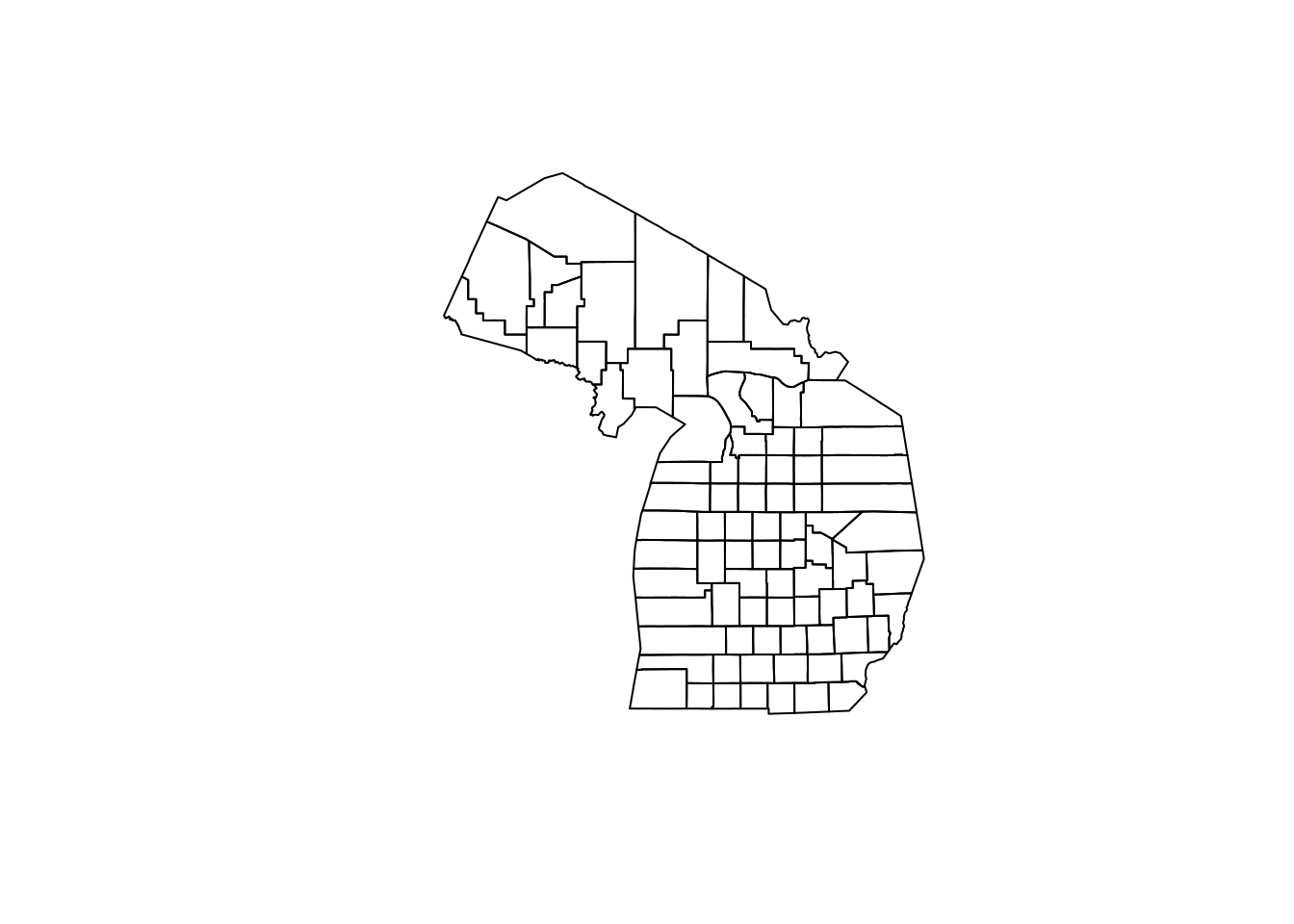
The census offers two types of boundaries. TIGER/LINE boundaries are contiguous and may span over water, while cartographic boundaries are simplified representations of selected geographic areas that only span over land.
cb = FALSE
MI_counties <- counties(state = "MI", year = 2020)plot(st_geometry(MI_counties))
cb = TRUE
MI_counties <- counties(state = "MI", year = 2020, cb = TRUE)plot(st_geometry(MI_counties))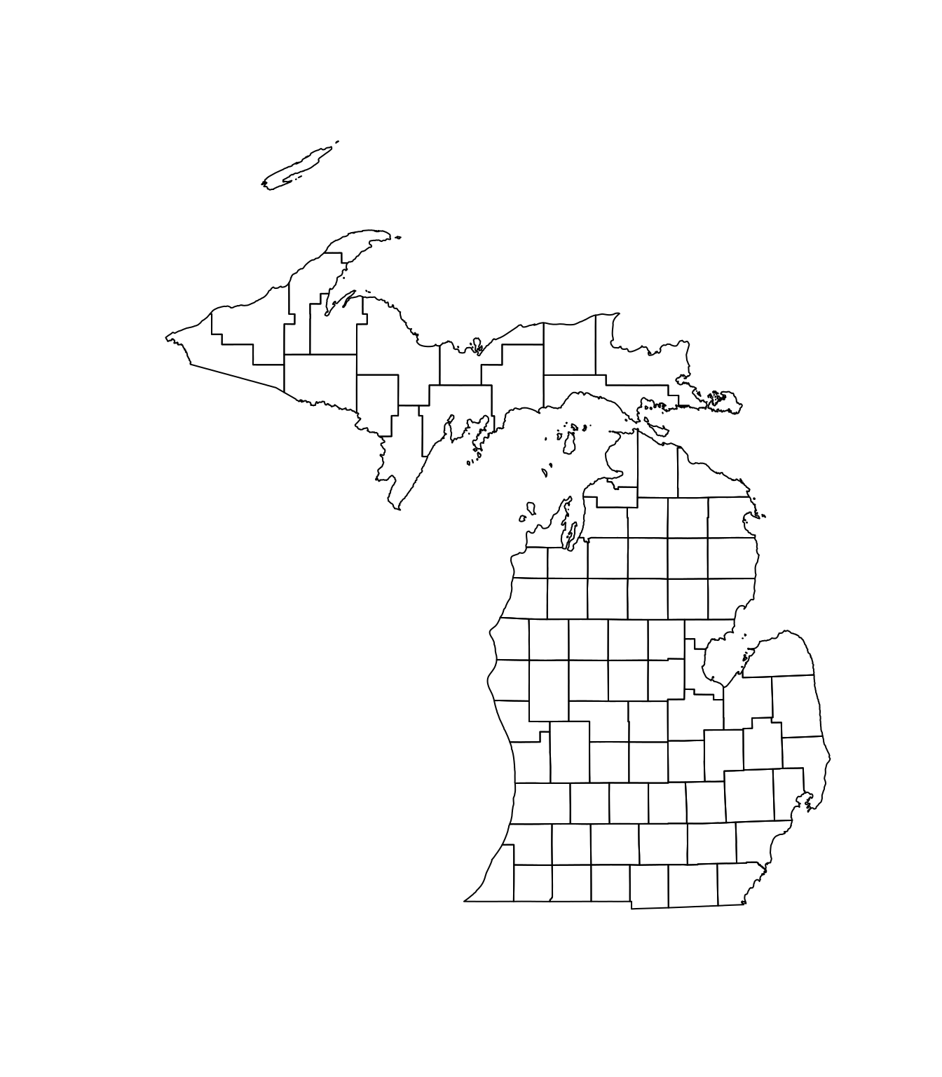
Writing Data
Writing data is just as easy as reading it. Use the st_write() function to write datasets. If you are having issues writing data, use st_drivers() to check the capabilities of your current drivers. Older drivers can not write geodatabases.
st_write(AZ_Hospitals, "data/AZ_Hospitals.shp")
# or
st_write(AZ_StatAreas, "data/file_path.gdb", layer = "layer_name")Visualizing Spatial Data
Projections
It is important to remember when making any 2 dimensional representation of a geographic area that the world is not flat. As a result, there are many different ways that we can represent the three dimensional space that our world inhabits within two dimensions. This problem is most pronounced when looking at larger areas.
The ways we transform three dimensional space into two dimensional representations are called projections. It is impossible to make a two dimensional map without introducing distortion to some aspect of the representation. However, many projections optimize for a specific aspect of a map (area, distance, angles, etc.).
For example, if we look at the 50 states, using the default projection (North American Datum of 1983), we can see that the US looks slightly different than we may be use to viewing it.
US_states <- states(cb = TRUE, year = 2020) %>%
filter(GEOID < "60") %>%
st_shift_longitude()
plot(st_geometry(US_states))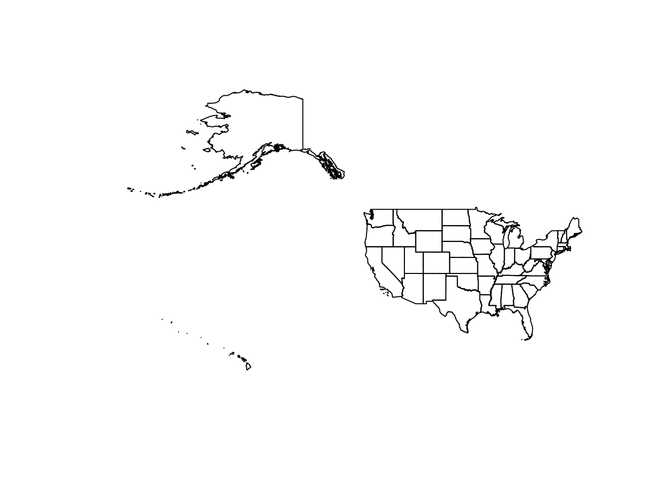
We can check the projection of our data using st_crs().
st_crs(US_states)Coordinate Reference System:
User input: NAD83
wkt:
GEOGCRS["NAD83",
DATUM["North American Datum 1983",
ELLIPSOID["GRS 1980",6378137,298.257222101,
LENGTHUNIT["metre",1]]],
PRIMEM["Greenwich",0,
ANGLEUNIT["degree",0.0174532925199433]],
CS[ellipsoidal,2],
AXIS["latitude",north,
ORDER[1],
ANGLEUNIT["degree",0.0174532925199433]],
AXIS["longitude",east,
ORDER[2],
ANGLEUNIT["degree",0.0174532925199433]],
ID["EPSG",4269]]We can transform our data into a different projection using st_transform().
Beware that projections are often accurate for certain geographic regions. For example, if we transform the 50 state’s projection to USA Contiguous Albers Equal Area Conic (ESRI:102003), we can see that the lower 48 states look as we might expect, while the Alaska and Hawaii look quite off.
US_states <- US_states %>%
st_transform("ESRI:102003")
plot(st_geometry(US_states))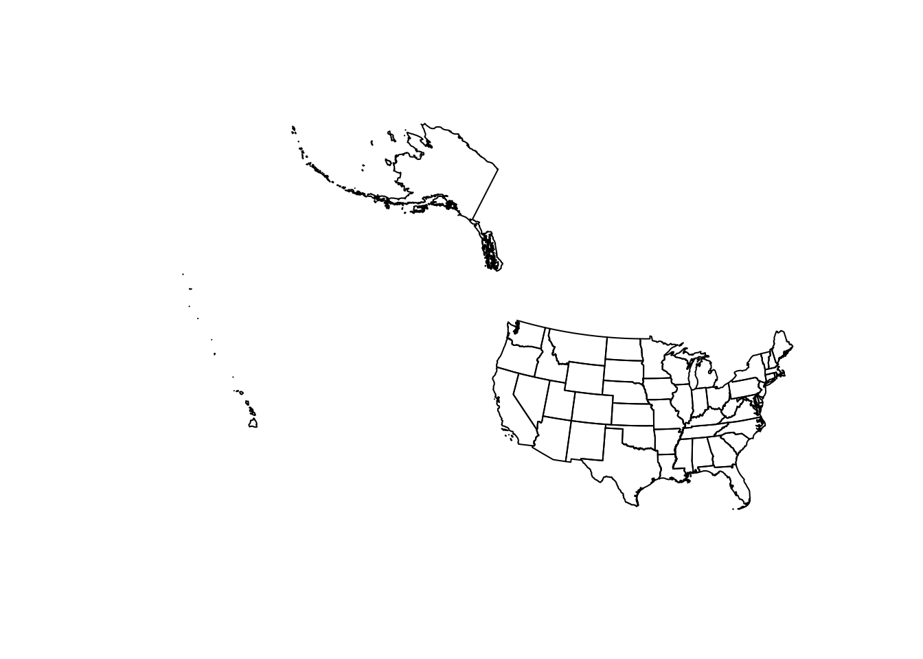
When trying to map all 50 states, we recommend using the tigris function shift_geometry(), which will shift and rescale Alaska, and Hawaii (and Puerto Rico if you include it) for thematic mapping.
US_states <- US_states %>%
shift_geometry()
ggplot() +
geom_sf(data = US_states)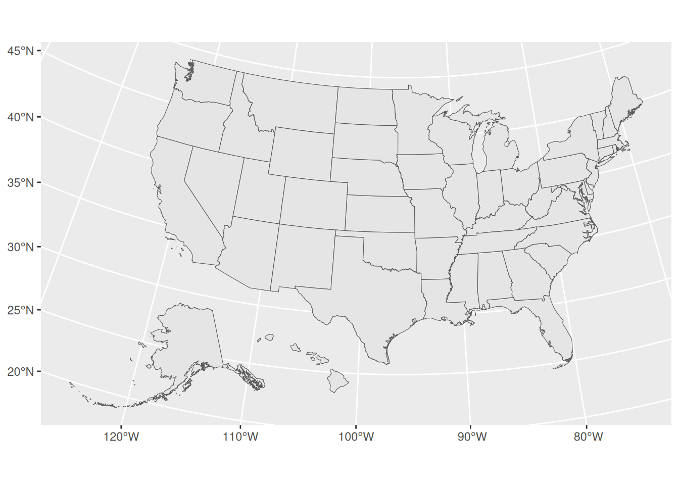
plot
The easiest way to look at any geography is through the default plot() function. plot() is not super customizable and hence is not the primary way most visualize spatial data within R. By default it will plot up to 9 of the columns within the sf object. We can select just the geometry column of an sf object using the st_geometry() function.
plot(st_geometry(AZ_StatAreas))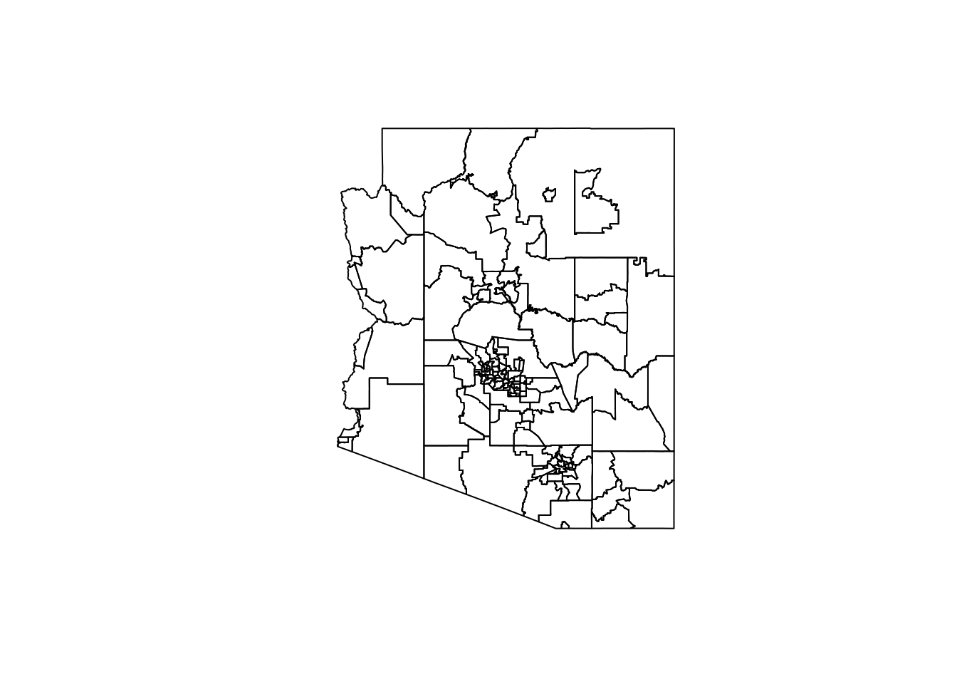
You can even add layers additonal layers to your plot using add = TRUE
plot(st_geometry(AZ_StatAreas))
plot(st_geometry(AZ_Hospitals), col = "red", pch = 19, cex = 0.5, add = TRUE)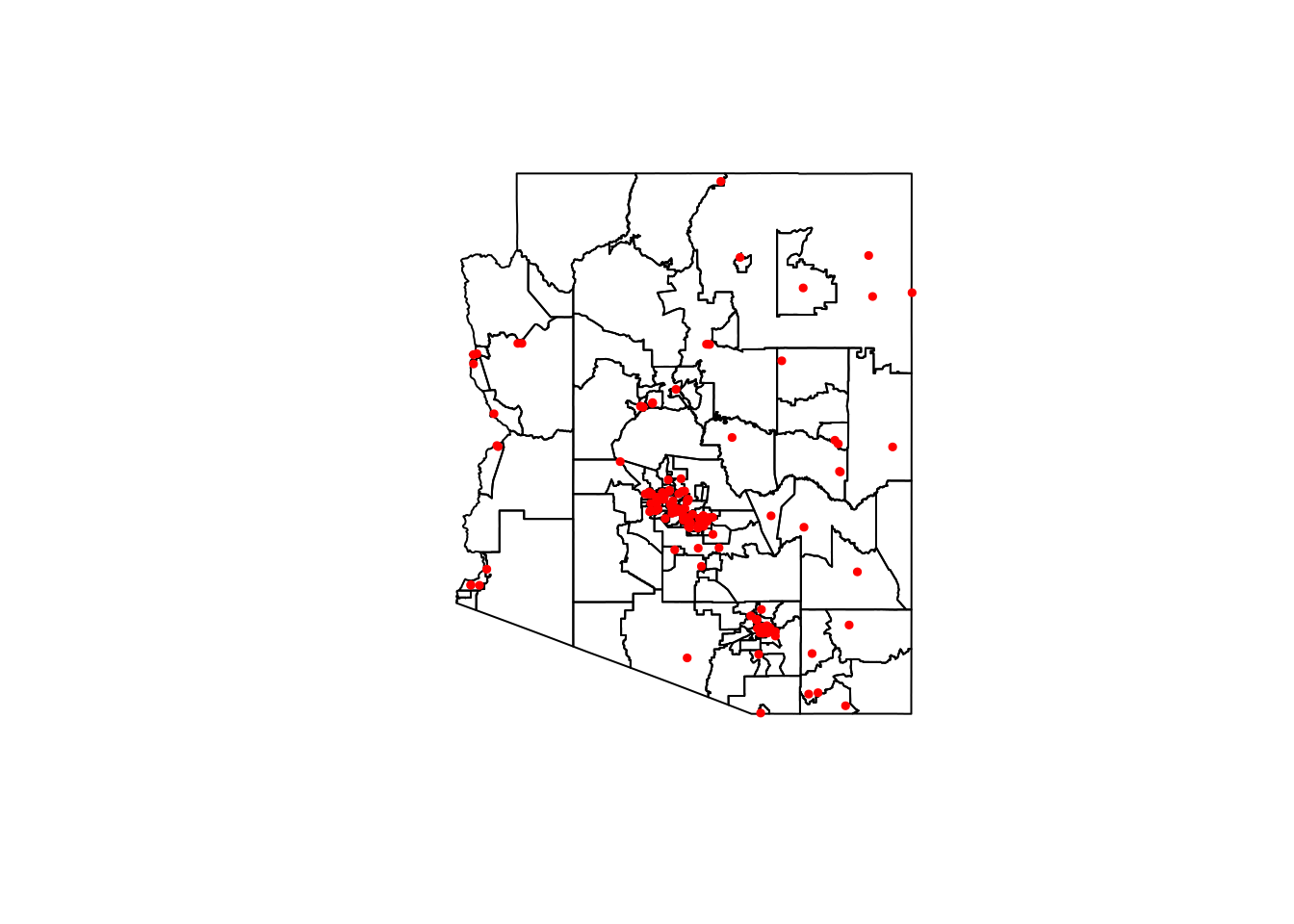
ggplot2
ggplot2 is the predominant data visualization package within R. Thankfully, you can use all the same syntax that you may have learned through using ggplot2 for non-spatial data to create beautiful maps. Simply use the geom_sf() function and specify your data.
Note
If you need more information about ggplot2, check out ggplot2: Elegant Graphics for Data Analysis
library(ggplot2)
ggplot() +
geom_sf(data = AZ_StatAreas) +
geom_sf(data = AZ_Hospitals, color = "red", size = 0.5)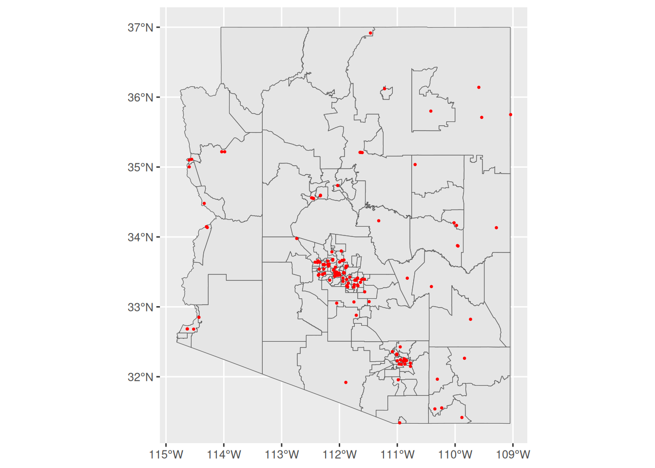
leaflet
Statics maps are only one way to visualize spatial data. Often we may have data that we want an audience to be able to play around with and explore. For this, we have interactive maps. Within R, the most comprehensive interactive mapping functionality is provided within the leaflet package.
leaflet can get quite complicated when you start adding options like - Popups/Labels - User controlled showing or hiding of layers - Custom markers - Custom legend text - Basemaps
As always, its important to think about whether that additional effort provides additional utility to the reader.
library(leaflet)
US_states <- states(cb = TRUE, year = 2020) %>%
filter(GEOID < "60")
US_interactive_map <- leaflet(US_states) %>%
addProviderTiles("CartoDB.Positron") %>%
addPolygons(
fillColor = "seagreen",
fillOpacity = 0.7,
color = "black",
weight = 0.5,
group = "states",
highlightOptions = highlightOptions(
color = "Black",
fillOpacity = 1,
bringToFront = T),
label = str_glue_data(US_states, "<strong>{NAME}</strong><br>FIPS Code: {GEOID}") %>%
map(htmltools::HTML),
) %>%
setView(-98.5795, 39.8282, zoom = 3)
US_interactive_mapDifferent Map Types
So far we have cover how to make basic maps visualizing geometry, but often we will want to represent data values visually. The follow maps allow us to visualize data in various ways.
Choropleths
Choropleths vary color of geographic regions based on a variable of interest. They are the most common type of map used within geospatial visualizations and offer an easy way to visualize how a variable varies across geographic regions.
When setting the fill of geographic regions, we use the following three functions
scale_fill_distiller- for continuous datascale_fill_brewer- for discrete data (factors or strings)scale_fill_fermenter- for continuous data we would like to bin
Continuous Scale
By default, ggplot will use a continuous scale to assign map variables onto colors.
AZ_PLACES_hosp <- st_read("data/pres/sample.geojson", as_tibble = TRUE)cont_map <- ggplot() +
geom_sf(data = AZ_PLACES_hosp, aes(fill = `Diabetes Adjusted Prevalence`)) +
scale_fill_distiller(palette = "Blues", direction = 1) +
labs(
title = "Diabetes Prevalence among Arizona Counties",
fill = "Diabetes Adjusted Prevalence \nAmong Adults >=18",
) +
theme_void()
cont_map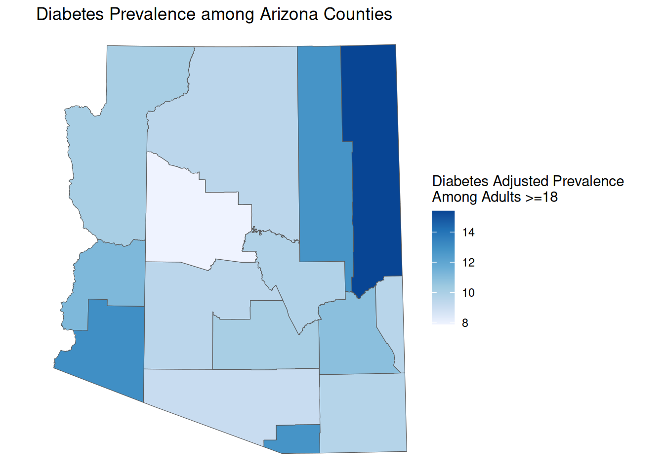
Quantile Breaks
For readers, it is often difficult to identify a color value and associate it with its value on the scale. Thefore, it is often a good choice to bin values into discrete groups. There are many ways to conduct binning. One of the most ubiquitous is quantiles. Quantile maps are great for making comparisons because you they allow you to compare quantiles across variables. However, they can have the effect of grouping widely different values.
quant_map <- ggplot() +
geom_sf(
data = AZ_PLACES_hosp,
aes(fill =
fct_rev(cut(
`Diabetes Adjusted Prevalence`,
quantile(
`Diabetes Adjusted Prevalence`,
probs = seq(0, 1, 0.2)),
include.lowest=TRUE)))) +
scale_fill_brewer(palette = "Blues", direction = -1) +
labs(
title = "Diabetes Prevalence among Arizona Counties",
fill = "Diabetes Adjusted Prevalence \nAmong Adults >=18",
) +
theme_void()
quant_map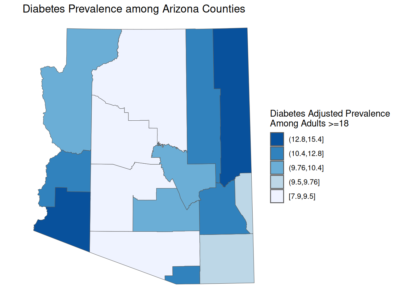
Equal Interval Breaks
You can also set equally sized breaks. This ends up being similar to a continuous color scale, but allows the reader to more easily identify values from their color.
equal_map <- ggplot() +
geom_sf(
data = AZ_PLACES_hosp,
aes(fill = `Diabetes Adjusted Prevalence`)
) +
scale_fill_fermenter(palette = "Blues", direction = 1) +
labs(
title = "Diabetes Prevalence among Arizona Counties",
fill = "Diabetes Adjusted Prevalence \nAmong Adults >=18",
) +
theme_void()
equal_map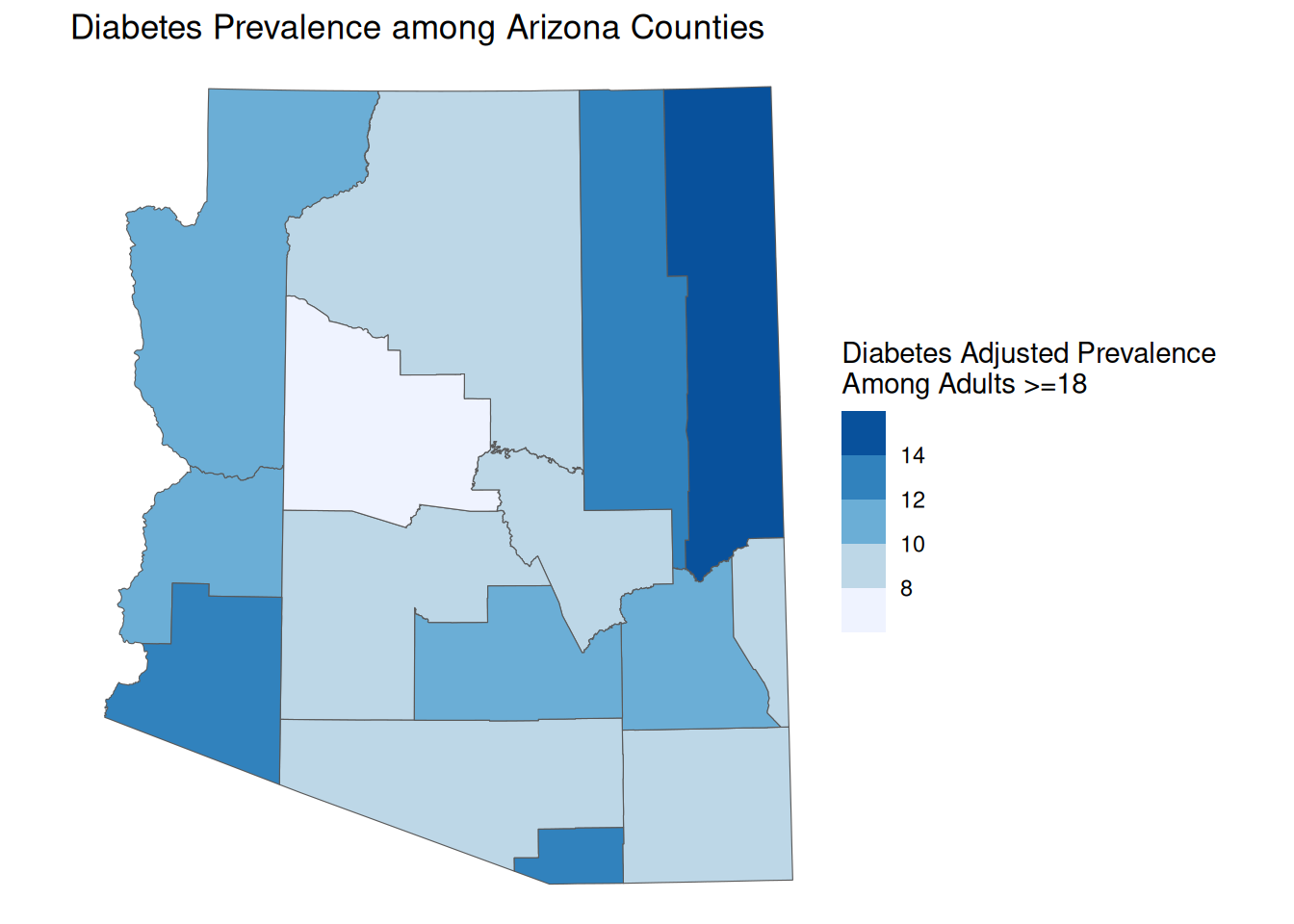
Manual Breaks
If you have prior knowledge of a dataset and an idea of what may compose meaningful breaks, you can also set manual breaks. This means you can also use your own classification method if you have another you prefer.
manual_map <- ggplot() +
geom_sf(
data = AZ_PLACES_hosp,
aes(fill = `Diabetes Adjusted Prevalence`)
) +
scale_fill_fermenter(palette = "Blues", direction = 1, breaks = c(9, 11, 13, 15)) +
labs(
title = "Diabetes Prevalence among Arizona Counties",
fill = "Diabetes Adjusted Prevalence \nAmong Adults >=18",
) +
theme_void()
manual_map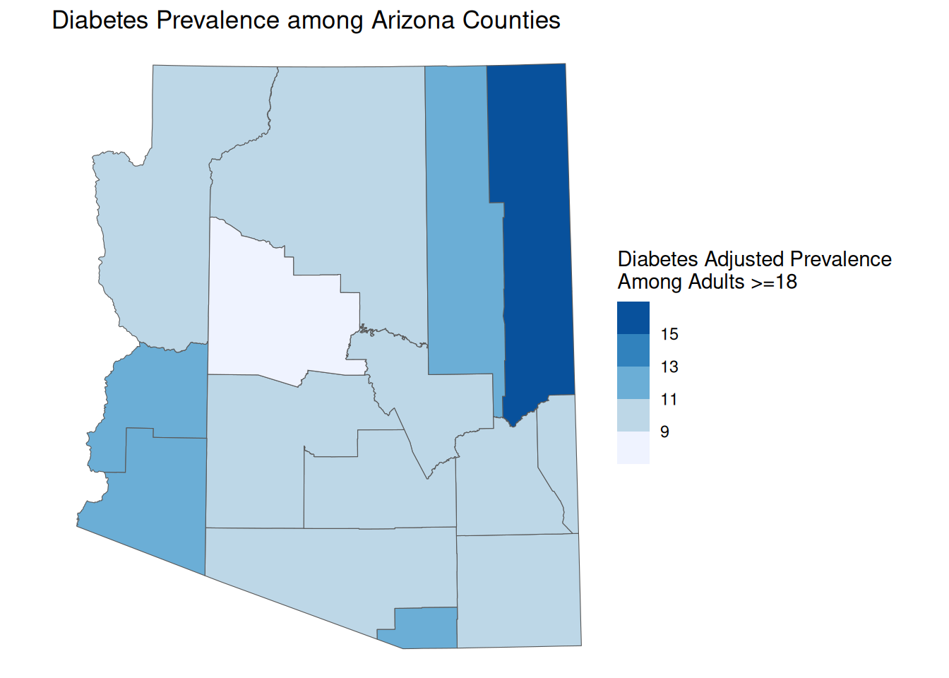
Comparisons of Breaks
To compare our breaks, we will use the plot_grid() function from cowplot to place our maps within a grid.
library(cowplot)
plot_grid(cont_map, quant_map, equal_map, manual_map)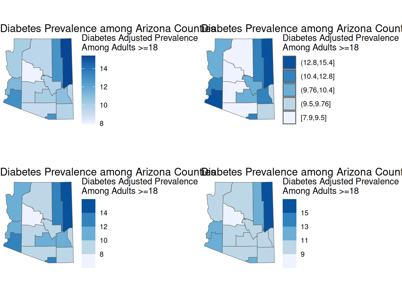
We can see that although our maps are all based off of the same data, we can get pretty different maps. This underscores the importance of using a good choice of breaks.
You are also not limited to the break methods listed above. There are several other break methods.
Cartograms
As a visual tool, choropleths are great, but they do have some faults. As viewers, we tend to associate larger areas with more importance, but often area is not correlated with population. Cartograms address this by transforming geographic areas so that their area is proportional to the population.
We can create a cartogram using the cartogram package. There are three different forms of cartograms that the package offers
- Continuous cartograms (
cartogram_cont) - distorts shape
- Discontinuous cartograms (
cartogram_ncont) - maintains shape, distorts size
- Dorling cartogram (
cartogram_dorling) - creates circles of weighted size
library(cartogram)
AZ_PLACES_hosp_carto <- AZ_PLACES_hosp %>%
cartogram_ncont("Population")ggplot() +
geom_sf(
data = AZ_PLACES_hosp_carto,
aes(fill = `Diabetes Adjusted Prevalence`)
) +
scale_fill_distiller(palette = "Blues", direction = -1) +
labs(
title = "Diabetes Prevalence among Arizona Counties",
fill = "Diabetes Adjusted Prevalence \nAmong Adults >=18",
) +
theme_void()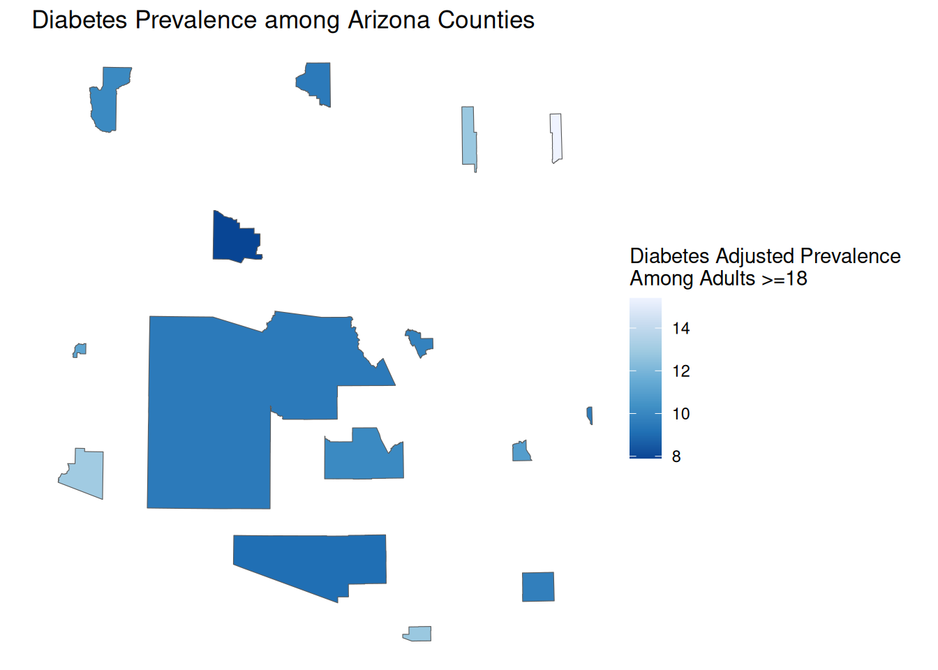
Proportional/Graduated Symbol Maps
Choropleths are best used with relative data (aka rates), but we typically use another form of map for count data, symbol maps. Like cartograms, symbol maps mitigate area bias, but allow us to avoid distorting the original area.
By default ggplot will use proportional symbols, which often have the same drawbacks as continuous choropleth maps. In order to create proportional symbols, we first need to calculate the center of each geographic region, which we can do using st_centroid(), and then we can change the size of the symbol based on our variable of choice.
We can also aggregate point locations to a geometry in order to mask the point locations. This is often important for location data that is sensitive.
Note
It is possible for some geographies that the centroid is placed outside of the geometry itself. If this is a concern for you, you can switch out st_centroid() for st_point_on_surface(), which will guarantee that the point is placed within the geometry.
ggplot() +
geom_sf(data = AZ_PLACES_hosp) +
geom_sf(
data = st_centroid(AZ_PLACES_hosp),
pch = 20,
aes(size = `Hospital Count`),
fill = alpha("red", 0.7),
col = "red"
) +
scale_size(range = c(1, 30)) +
labs(
title = "Hospital Count by County",
size = "Number of Hospitals",
) +
theme_void()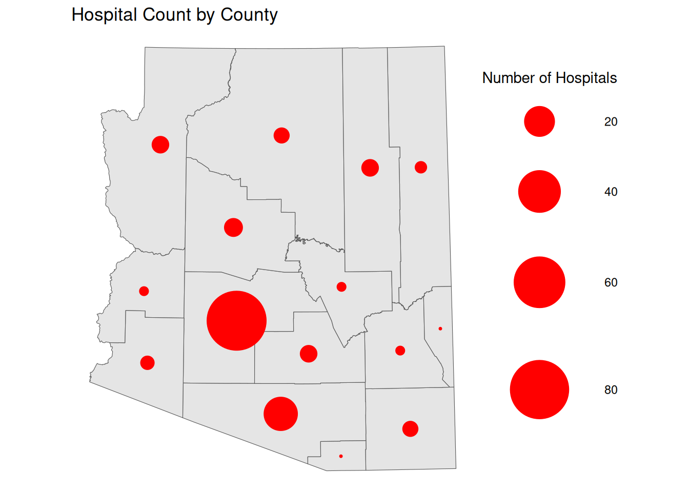
Just like choropleth maps, we can bin our data to create graduated symbols.
ggplot() +
geom_sf(data = AZ_PLACES_hosp) +
geom_sf(
data = st_centroid(AZ_PLACES_hosp),
pch = 20,
aes(size = `Hospital Count`),
fill = alpha("red", 0.7),
col = "red"
) +
scale_size_binned(range = c(1, 30), breaks = c(5, 10, 20)) +
labs(
title = "Hospital Count by County",
size = "Number of Hospitals",
) +
theme_void()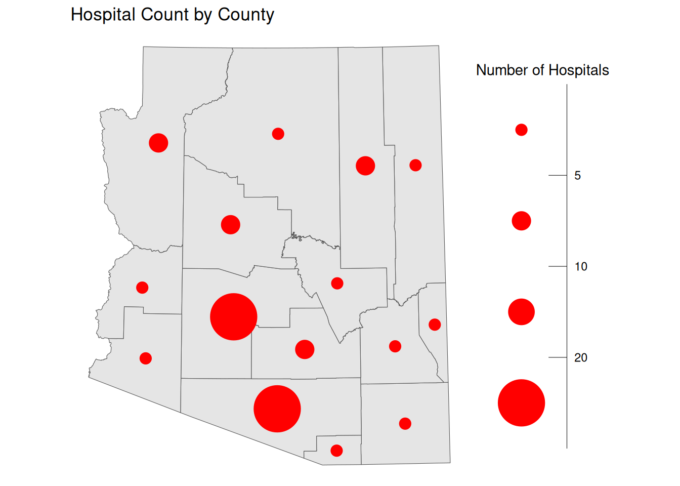
Dot Density
Another way to visualize counts is through the use of dot density maps. Dot density maps randomly distribute dots through out geographic area to display counts. Often, each dot will represent some count value. If you have sensitive location data, you can also use a dot density map to mask the locations, while still giving the viewer some idea of where the locations lie.
We can use the as_dot_density function from the tidycensus package to create a dot density map for us.
library(tidycensus)
AZ_pop_dots <- as_dot_density(
AZ_PLACES_hosp,
value = "Population",
values_per_dot = 10000,
group = "GEOID"
)
ggplot() +
geom_sf(data = AZ_PLACES_hosp) +
geom_sf(data = AZ_pop_dots) +
labs(
title = "Arizona Population by County",
caption = "1 dot = 10000"
) +
theme_void()Geocomputation
More on Projections
Much of the data you may come across will be unprojected. In R, you can check if an sf object is unprojected by using st_is_longlat(). For unprojected data, R uses a geocomputing engine called S2 which represents the earth which approximates the earth as a sphere. S2 is great an mitigates potential issues associated with the planar assumption, but S2 is not perfect. We often find that using a good projection can reduce frustrations when conducting geocomputation.
The following figure shows how unprojected data assumes that a degree is a uniform distance, when this is not the case, as the projected data more clearly shows.
US_states <- states() %>%
filter(GEOID < "60")
unprojected <- ggplot() +
geom_sf(data = US_states)
projected <- ggplot() +
geom_sf(data = st_transform(US_states, "ESRI:102003"))
plot_grid(projected, unprojected, labels = c('projected', 'unprojected'))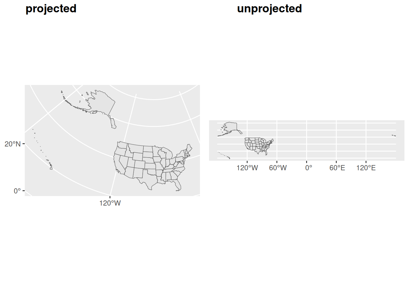
Typical Identifiers
Some geocomputation operations rely on a unique identifier. For example, Census geographies are uniquely identified by FIPS Codes (aka GEOIDs).
The following table breaks down the structure of FIPS codes some of the major Census geographies. For more information on FIPS codes check out the Census Reference.
| Area | Structure | Digits |
|---|---|---|
| State | STATE | 2 |
| County | STATE+COUNTY | 2+3=5 |
| Tract | STATE+COUNTY+TRACT | 2+3+6=11 |
| Block Group | STATE+COUNTY+TRACT+BLOCK GROUP | 2+3+6+1=12 |
| Block | STATE+COUNTY+TRACT+BLOCK | 2+3+6+4=15 |
Tabular Joins
One of the most common operations that we may need to conduct is connecting a spatial dataset to a table using join. As we talked about before, sf objects are simply data.frames or tibbles with an extra geometry column. Fortunately, this means we can use all the typical tidyverse functions for joining tables (left_join(), right_join(), inner_join(), outer_join(), etc.).
These joins rely on at least one unique identifier that is present in both tables. If you are having problems joining tables, make sure that the data type of the unique identifier is the same amongst the two tables.
states <- counties(state = "AZ") %>%
select(GEOID)
PLACES <- read_csv("data/US/PLACES2023/PLACES2023_county.csv")
left_join(states, PLACES, join_by(GEOID == CountyFIPS))| GEOID | StateAbbr | StateDesc | CountyName | TotalPopulation | ACCESS2_CrudePrev | ACCESS2_Crude95CI | ACCESS2_AdjPrev | ACCESS2_Adj95CI | ARTHRITIS_CrudePrev | ARTHRITIS_Crude95CI | ARTHRITIS_AdjPrev | ARTHRITIS_Adj95CI | BINGE_CrudePrev | BINGE_Crude95CI | BINGE_AdjPrev | BINGE_Adj95CI | BPHIGH_CrudePrev | BPHIGH_Crude95CI | BPHIGH_AdjPrev | BPHIGH_Adj95CI | BPMED_CrudePrev | BPMED_Crude95CI | BPMED_AdjPrev | BPMED_Adj95CI | CANCER_CrudePrev | CANCER_Crude95CI | CANCER_AdjPrev | CANCER_Adj95CI | CASTHMA_CrudePrev | CASTHMA_Crude95CI | CASTHMA_AdjPrev | CASTHMA_Adj95CI | CERVICAL_CrudePrev | CERVICAL_Crude95CI | CERVICAL_AdjPrev | CERVICAL_Adj95CI | CHD_CrudePrev | CHD_Crude95CI | CHD_AdjPrev | CHD_Adj95CI | CHECKUP_CrudePrev | CHECKUP_Crude95CI | CHECKUP_AdjPrev | CHECKUP_Adj95CI | CHOLSCREEN_CrudePrev | CHOLSCREEN_Crude95CI | CHOLSCREEN_AdjPrev | CHOLSCREEN_Adj95CI | COLON_SCREEN_CrudePrev | COLON_SCREEN_Crude95CI | COLON_SCREEN_AdjPrev | COLON_SCREEN_Adj95CI | COPD_CrudePrev | COPD_Crude95CI | COPD_AdjPrev | COPD_Adj95CI | COREM_CrudePrev | COREM_Crude95CI | COREM_AdjPrev | COREM_Adj95CI | COREW_CrudePrev | COREW_Crude95CI | COREW_AdjPrev | COREW_Adj95CI | CSMOKING_CrudePrev | CSMOKING_Crude95CI | CSMOKING_AdjPrev | CSMOKING_Adj95CI | DENTAL_CrudePrev | DENTAL_Crude95CI | DENTAL_AdjPrev | DENTAL_Adj95CI | DEPRESSION_CrudePrev | DEPRESSION_Crude95CI | DEPRESSION_AdjPrev | DEPRESSION_Adj95CI | DIABETES_CrudePrev | DIABETES_Crude95CI | DIABETES_AdjPrev | DIABETES_Adj95CI | GHLTH_CrudePrev | GHLTH_Crude95CI | GHLTH_AdjPrev | GHLTH_Adj95CI | HIGHCHOL_CrudePrev | HIGHCHOL_Crude95CI | HIGHCHOL_AdjPrev | HIGHCHOL_Adj95CI | KIDNEY_CrudePrev | KIDNEY_Crude95CI | KIDNEY_AdjPrev | KIDNEY_Adj95CI | LPA_CrudePrev | LPA_Crude95CI | LPA_AdjPrev | LPA_Adj95CI | MAMMOUSE_CrudePrev | MAMMOUSE_Crude95CI | MAMMOUSE_AdjPrev | MAMMOUSE_Adj95CI | MHLTH_CrudePrev | MHLTH_Crude95CI | MHLTH_AdjPrev | MHLTH_Adj95CI | OBESITY_CrudePrev | OBESITY_Crude95CI | OBESITY_AdjPrev | OBESITY_Adj95CI | PHLTH_CrudePrev | PHLTH_Crude95CI | PHLTH_AdjPrev | PHLTH_Adj95CI | SLEEP_CrudePrev | SLEEP_Crude95CI | SLEEP_AdjPrev | SLEEP_Adj95CI | STROKE_CrudePrev | STROKE_Crude95CI | STROKE_AdjPrev | STROKE_Adj95CI | TEETHLOST_CrudePrev | TEETHLOST_Crude95CI | TEETHLOST_AdjPrev | TEETHLOST_Adj95CI | HEARING_CrudePrev | HEARING_Crude95CI | HEARING_AdjPrev | HEARING_Adj95CI | VISION_CrudePrev | VISION_Crude95CI | VISION_AdjPrev | VISION_Adj95CI | COGNITION_CrudePrev | COGNITION_Crude95CI | COGNITION_AdjPrev | COGNITION_Adj95CI | MOBILITY_CrudePrev | MOBILITY_Crude95CI | MOBILITY_AdjPrev | MOBILITY_Adj95CI | SELFCARE_CrudePrev | SELFCARE_Crude95CI | SELFCARE_AdjPrev | SELFCARE_Adj95CI | INDEPLIVE_CrudePrev | INDEPLIVE_Crude95CI | INDEPLIVE_AdjPrev | INDEPLIVE_Adj95CI | DISABILITY_CrudePrev | DISABILITY_Crude95CI | DISABILITY_AdjPrev | DISABILITY_Adj95CI | Geolocation | geometry |
|---|---|---|---|---|---|---|---|---|---|---|---|---|---|---|---|---|---|---|---|---|---|---|---|---|---|---|---|---|---|---|---|---|---|---|---|---|---|---|---|---|---|---|---|---|---|---|---|---|---|---|---|---|---|---|---|---|---|---|---|---|---|---|---|---|---|---|---|---|---|---|---|---|---|---|---|---|---|---|---|---|---|---|---|---|---|---|---|---|---|---|---|---|---|---|---|---|---|---|---|---|---|---|---|---|---|---|---|---|---|---|---|---|---|---|---|---|---|---|---|---|---|---|---|---|---|---|---|---|---|---|---|---|---|---|---|---|---|---|---|---|---|---|---|---|---|---|---|---|---|---|---|---|---|---|
| 04027 | AZ | Arizona | Yuma | 206990 | 23.6 | (18.6, 29.5) | 23.7 | (18.8, 29.4) | 22.9 | (20.0, 26.0) | 20.0 | (17.3, 22.9) | 15.9 | (13.3, 18.7) | 17.2 | (14.4, 20.3) | 33.3 | (29.9, 36.7) | 30.2 | (26.9, 33.6) | 77.2 | (74.2, 79.8) | 57.3 | (52.7, 62.0) | 6.9 | ( 6.2, 7.6) | 5.5 | ( 5.0, 6.1) | 9.7 | ( 8.6, 11.0) | 9.9 | ( 8.7, 11.1) | 76.4 | (73.5, 79.0) | 77.7 | (75.1, 80.2) | 7.6 | ( 6.7, 8.7) | 6.1 | ( 5.3, 6.9) | 67.6 | (63.1, 72.1) | 65.5 | (60.7, 70.2) | 80.7 | (77.5, 83.8) | 80.0 | (76.5, 83.2) | 63.2 | (60.5, 65.7) | 59.8 | (56.7, 62.6) | 7.4 | ( 6.1, 8.7) | 6.4 | ( 5.4, 7.5) | 36.3 | (30.1, 42.5) | 36.2 | (30.1, 42.3) | 29.0 | (24.3, 34.1) | 29.2 | (24.3, 34.2) | 14.5 | (11.9, 17.4) | 15.7 | (12.9, 18.8) | 52.3 | (48.7, 56.0) | 51.7 | (47.8, 55.6) | 17.9 | (15.0, 21.0) | 18.4 | (15.4, 21.6) | 14.3 | (12.4, 16.3) | 13.0 | (11.3, 14.8) | 23.2 | (20.0, 26.8) | 22.4 | (19.3, 25.9) | 36.3 | (32.6, 40.1) | 31.2 | (27.4, 35.1) | 4.2 | ( 3.8, 4.6) | 3.6 | ( 3.2, 3.9) | 31.2 | (27.0, 36.1) | 30.5 | (26.1, 35.2) | 65.2 | (61.4, 68.8) | 66.2 | (62.3, 69.9) | 15.8 | (13.6, 18.1) | 16.4 | (14.2, 18.8) | 39.1 | (33.6, 44.9) | 40.8 | (35.1, 46.7) | 14.1 | (12.1, 16.1) | 13.5 | (11.6, 15.5) | 35.1 | (33.9, 36.3) | 36.6 | (35.3, 37.9) | 4.0 | ( 3.5, 4.5) | 3.3 | ( 2.9, 3.7) | 13.7 | ( 9.9, 17.8) | 14.6 | (10.7, 18.9) | 9.1 | ( 8.1, 10.2) | 7.4 | ( 6.6, 8.3) | 8.2 | ( 7.1, 9.5) | 7.8 | ( 6.7, 9.0) | 16.3 | (13.9, 19.0) | 16.5 | (14.1, 19.2) | 16.9 | (14.6, 19.3) | 15.0 | (12.8, 17.2) | 5.5 | ( 4.7, 6.3) | 5.2 | ( 4.5, 6.0) | 9.6 | ( 8.3, 11.1) | 9.2 | ( 7.9, 10.6) | 33.3 | (28.9, 37.6) | 30.9 | (26.7, 35.1) | POINT (-113.910905 32.7739424) | MULTIPOLYGON (((-114.8141 3… |
| 04021 | AZ | Arizona | Pinal | 449557 | 14.1 | (11.5, 17.0) | 14.5 | (11.8, 17.5) | 28.1 | (25.2, 30.9) | 23.5 | (21.0, 26.2) | 16.3 | (13.8, 18.8) | 18.2 | (15.5, 21.0) | 33.0 | (29.9, 36.0) | 28.5 | (25.6, 31.4) | 77.0 | (73.9, 79.7) | 55.8 | (51.4, 60.0) | 7.8 | ( 7.0, 8.5) | 6.1 | ( 5.5, 6.7) | 10.0 | ( 8.8, 11.2) | 10.1 | ( 8.9, 11.4) | 79.4 | (77.0, 81.3) | 79.8 | (77.7, 81.7) | 7.0 | ( 6.1, 8.0) | 5.4 | ( 4.8, 6.2) | 71.6 | (67.8, 75.2) | 68.8 | (64.8, 72.7) | 83.3 | (80.7, 85.8) | 80.9 | (77.9, 83.7) | 68.8 | (66.6, 71.1) | 64.9 | (62.5, 67.4) | 7.6 | ( 6.3, 9.0) | 6.3 | ( 5.3, 7.5) | 44.8 | (38.3, 51.1) | 44.7 | (38.3, 50.8) | 37.6 | (31.7, 43.4) | 36.7 | (31.1, 42.1) | 16.6 | (13.8, 19.6) | 17.2 | (14.2, 20.2) | 53.9 | (50.8, 56.9) | 53.2 | (50.0, 56.0) | 17.9 | (15.3, 20.5) | 18.5 | (15.8, 21.3) | 12.1 | (10.6, 13.8) | 10.1 | ( 8.9, 11.5) | 18.4 | (15.7, 21.2) | 17.2 | (14.6, 19.8) | 37.7 | (34.4, 41.0) | 31.3 | (27.9, 34.6) | 3.7 | ( 3.3, 4.1) | 3.1 | ( 2.8, 3.3) | 25.4 | (21.7, 29.3) | 24.3 | (20.7, 27.9) | 66.1 | (62.4, 69.8) | 67.1 | (63.5, 70.5) | 15.0 | (13.1, 16.9) | 16.0 | (14.1, 18.0) | 37.2 | (32.6, 41.9) | 37.5 | (32.9, 42.2) | 12.9 | (11.2, 14.8) | 12.0 | (10.4, 13.6) | 35.7 | (34.6, 36.8) | 37.0 | (35.8, 38.0) | 3.6 | ( 3.2, 4.1) | 2.9 | ( 2.6, 3.3) | 12.8 | ( 8.9, 17.5) | 13.2 | ( 9.3, 18.3) | 8.2 | ( 7.2, 9.2) | 6.7 | ( 6.0, 7.5) | 5.4 | ( 4.7, 6.3) | 5.1 | ( 4.4, 5.9) | 13.8 | (11.8, 15.8) | 14.4 | (12.3, 16.5) | 14.9 | (12.8, 17.2) | 12.6 | (10.9, 14.6) | 4.0 | ( 3.5, 4.6) | 3.7 | ( 3.2, 4.2) | 7.8 | ( 6.6, 8.9) | 7.5 | ( 6.4, 8.7) | 31.0 | (27.0, 34.7) | 28.8 | (25.1, 32.4) | POINT (-111.3663396 32.9185209) | MULTIPOLYGON (((-111.2669 3… |
| 04017 | AZ | Arizona | Navajo | 108147 | 14.6 | (12.1, 17.7) | 15.3 | (12.7, 18.5) | 29.8 | (26.7, 32.8) | 24.9 | (22.2, 27.6) | 14.7 | (12.4, 17.1) | 16.6 | (14.0, 19.3) | 37.3 | (33.9, 40.5) | 32.3 | (29.1, 35.3) | 77.3 | (74.4, 80.0) | 56.6 | (52.3, 60.9) | 7.7 | ( 6.9, 8.5) | 6.1 | ( 5.5, 6.7) | 12.6 | (11.2, 14.0) | 12.8 | (11.4, 14.2) | 74.7 | (72.5, 76.9) | 75.7 | (73.5, 77.8) | 9.0 | ( 8.0, 10.2) | 7.1 | ( 6.3, 8.0) | 68.8 | (64.8, 72.5) | 65.8 | (61.4, 69.8) | 79.1 | (76.1, 81.9) | 75.9 | (72.7, 79.2) | 59.9 | (57.6, 62.2) | 56.1 | (53.7, 58.4) | 10.7 | ( 9.1, 12.3) | 8.9 | ( 7.6, 10.2) | 31.0 | (25.8, 36.0) | 31.2 | (26.1, 36.4) | 22.1 | (18.2, 26.0) | 21.7 | (18.0, 25.5) | 20.9 | (17.6, 24.1) | 21.9 | (18.5, 25.3) | 52.9 | (49.8, 55.8) | 52.1 | (49.1, 55.2) | 20.3 | (17.4, 23.3) | 21.1 | (18.1, 24.1) | 15.4 | (13.5, 17.4) | 12.8 | (11.1, 14.4) | 24.2 | (21.2, 27.3) | 22.5 | (19.8, 25.3) | 36.2 | (32.8, 39.4) | 28.8 | (25.6, 32.0) | 4.6 | ( 4.2, 5.1) | 3.8 | ( 3.5, 4.2) | 27.1 | (23.2, 31.0) | 25.9 | (22.2, 29.6) | 57.4 | (53.8, 60.9) | 57.3 | (53.6, 60.7) | 18.7 | (16.4, 20.8) | 20.1 | (17.7, 22.4) | 38.0 | (33.0, 42.6) | 38.2 | (33.3, 42.9) | 16.5 | (14.5, 18.5) | 15.3 | (13.4, 17.1) | 37.7 | (36.5, 38.7) | 39.0 | (37.8, 40.0) | 5.0 | ( 4.4, 5.6) | 4.1 | ( 3.7, 4.5) | 17.4 | (13.4, 21.9) | 18.2 | (13.9, 22.9) | 10.5 | ( 9.4, 11.7) | 8.9 | ( 7.9, 9.8) | 8.6 | ( 7.5, 9.7) | 8.0 | ( 7.0, 9.0) | 18.4 | (16.0, 20.7) | 19.2 | (16.7, 21.6) | 20.1 | (17.7, 22.5) | 17.1 | (15.0, 19.2) | 6.3 | ( 5.5, 7.2) | 5.7 | ( 5.0, 6.4) | 11.7 | (10.2, 13.3) | 11.4 | (10.0, 12.9) | 37.8 | (33.8, 41.6) | 35.5 | (31.7, 39.4) | POINT (-110.3210248 35.3907852) | MULTIPOLYGON (((-110.0007 3… |
| 04011 | AZ | Arizona | Greenlee | 9404 | 16.2 | (12.9, 19.4) | 16.2 | (13.0, 19.5) | 21.2 | (17.8, 24.7) | 20.1 | (16.8, 23.5) | 18.1 | (14.9, 21.7) | 18.5 | (15.2, 22.2) | 27.0 | (23.3, 30.8) | 25.8 | (22.2, 29.5) | 72.5 | (68.7, 76.0) | 53.8 | (48.6, 58.8) | 6.1 | ( 5.5, 6.7) | 5.7 | ( 5.2, 6.3) | 9.7 | ( 8.5, 11.0) | 9.7 | ( 8.5, 11.0) | 78.5 | (76.3, 80.8) | 79.2 | (77.1, 81.4) | 5.5 | ( 4.8, 6.2) | 5.1 | ( 4.5, 5.8) | 64.1 | (58.2, 69.7) | 63.4 | (57.4, 69.0) | 81.3 | (78.0, 84.4) | 80.7 | (77.3, 84.0) | 63.1 | (60.7, 65.7) | 61.5 | (59.1, 64.1) | 5.5 | ( 4.7, 6.4) | 5.2 | ( 4.4, 6.1) | 34.0 | (27.9, 40.3) | 34.8 | (28.7, 40.8) | 30.0 | (24.9, 35.4) | 30.8 | (25.7, 36.2) | 14.9 | (12.1, 17.8) | 14.9 | (12.2, 17.9) | 56.7 | (53.5, 59.8) | 56.8 | (53.5, 59.9) | 18.3 | (14.9, 21.9) | 18.4 | (15.0, 22.1) | 10.1 | ( 8.6, 11.6) | 9.6 | ( 8.2, 11.0) | 16.4 | (14.1, 18.8) | 16.1 | (13.8, 18.5) | 30.8 | (26.6, 35.4) | 27.5 | (23.3, 32.2) | 3.2 | ( 2.9, 3.5) | 3.1 | ( 2.8, 3.4) | 23.3 | (19.2, 27.7) | 23.1 | (18.8, 27.5) | 67.8 | (64.1, 71.4) | 67.1 | (63.3, 71.0) | 15.3 | (13.2, 17.4) | 15.6 | (13.5, 17.7) | 31.1 | (24.2, 38.6) | 31.1 | (24.3, 38.5) | 11.2 | ( 9.7, 12.8) | 11.0 | ( 9.5, 12.4) | 33.4 | (32.1, 34.6) | 33.6 | (32.3, 34.9) | 2.9 | ( 2.6, 3.2) | 2.7 | ( 2.4, 3.0) | 10.7 | ( 7.7, 13.6) | 11.5 | ( 8.4, 14.8) | 6.7 | ( 5.9, 7.5) | 6.4 | ( 5.7, 7.1) | 5.2 | ( 4.5, 5.9) | 5.1 | ( 4.5, 5.8) | 13.5 | (11.5, 15.5) | 13.7 | (11.6, 15.7) | 12.2 | (10.5, 14.0) | 11.7 | (10.0, 13.4) | 3.6 | ( 3.2, 4.1) | 3.5 | ( 3.1, 4.0) | 6.9 | ( 6.0, 7.9) | 6.9 | ( 6.0, 7.9) | 27.6 | (23.7, 31.6) | 27.1 | (23.1, 31.1) | POINT (-109.2423231 33.2388723) | MULTIPOLYGON (((-109.4958 3… |
| 04013 | AZ | Arizona | Maricopa | 4496588 | 12.7 | (10.3, 15.3) | 12.9 | (10.4, 15.7) | 22.9 | (20.9, 25.0) | 21.1 | (19.2, 23.0) | 16.7 | (14.8, 18.6) | 17.4 | (15.5, 19.4) | 29.6 | (27.3, 31.9) | 27.7 | (25.5, 29.9) | 72.9 | (70.2, 75.3) | 53.8 | (50.5, 57.1) | 6.9 | ( 6.3, 7.5) | 6.2 | ( 5.7, 6.8) | 9.9 | ( 9.0, 11.0) | 10.0 | ( 9.0, 11.0) | 80.6 | (78.6, 82.6) | 81.2 | (79.2, 83.1) | 5.8 | ( 5.1, 6.6) | 5.2 | ( 4.6, 5.9) | 69.2 | (66.1, 72.0) | 68.0 | (64.8, 71.0) | 84.0 | (81.7, 86.3) | 83.3 | (80.8, 85.6) | 67.8 | (65.2, 70.2) | 66.1 | (63.3, 68.6) | 5.9 | ( 4.9, 7.0) | 5.4 | ( 4.5, 6.4) | 45.1 | (38.4, 51.0) | 45.3 | (38.8, 51.2) | 36.2 | (30.3, 41.5) | 36.0 | (30.3, 41.3) | 13.8 | (11.4, 16.3) | 14.0 | (11.5, 16.6) | 61.9 | (58.9, 64.9) | 61.7 | (58.7, 64.7) | 18.7 | (16.7, 20.9) | 18.9 | (16.9, 21.1) | 10.4 | ( 9.2, 11.5) | 9.5 | ( 8.5, 10.6) | 15.4 | (13.2, 17.6) | 14.8 | (12.8, 17.0) | 34.5 | (32.2, 36.9) | 30.6 | (28.2, 33.1) | 3.3 | ( 3.0, 3.6) | 3.0 | ( 2.7, 3.3) | 22.4 | (19.4, 25.5) | 22.0 | (19.0, 25.1) | 69.0 | (65.5, 72.3) | 69.1 | (65.7, 72.5) | 16.1 | (14.5, 17.8) | 16.5 | (14.8, 18.3) | 30.8 | (27.4, 34.3) | 30.9 | (27.6, 34.4) | 10.9 | ( 9.5, 12.3) | 10.5 | ( 9.2, 11.9) | 31.7 | (30.6, 32.7) | 32.2 | (31.1, 33.3) | 2.9 | ( 2.6, 3.3) | 2.7 | ( 2.4, 3.1) | 10.3 | ( 6.7, 14.7) | 10.8 | ( 7.1, 15.6) | 6.6 | ( 5.8, 7.3) | 6.1 | ( 5.4, 6.8) | 4.7 | ( 4.1, 5.3) | 4.5 | ( 3.9, 5.2) | 13.2 | (11.5, 15.1) | 13.4 | (11.6, 15.4) | 12.7 | (11.0, 14.5) | 11.8 | (10.2, 13.5) | 3.4 | ( 2.9, 4.0) | 3.3 | ( 2.8, 3.8) | 6.8 | ( 5.9, 7.9) | 6.7 | ( 5.8, 7.8) | 28.5 | (25.5, 31.5) | 27.6 | (24.7, 30.6) | POINT (-112.4989296 33.3451756) | MULTIPOLYGON (((-111.8931 3… |
Table to Points
It is common practice to send point data as a table with longitude and latitude fields. Because these tables are not saved in a spatial format, they must be first read as a table and then converted to a sf object. It is important that if you recieve a dataset like this, that you check the documentation to see what coordinate reference system your data refers to. It is common convention to use WGS 1984 (EPSG:4326), but this cannot always be assumed.
cop2020_tract <- read_csv("data/US/COP2020/COP2020_tract.txt")
st_as_sf(cop2020_tract, coords = c("LONGITUDE", "LATITUDE"), crs = 4326)| STATEFP | COUNTYFP | TRACTCE | POPULATION | geometry |
|---|---|---|---|---|
| 01 | 001 | 020100 | 1775 | POINT (-86.4866 32.47682) |
| 01 | 001 | 020200 | 2055 | POINT (-86.47259 32.4719) |
| 01 | 001 | 020300 | 3216 | POINT (-86.45925 32.47458) |
| 01 | 001 | 020400 | 4246 | POINT (-86.44299 32.46866) |
| 01 | 001 | 020501 | 4322 | POINT (-86.42442 32.45153) |
Spatial Joins
Spatial joins allow us to conduct a join based on a spatial relationship. In practice this means that we can combine the attribute tables of two spatial datasets. sf offers us a plethora of spatial relationships to pick from including like st_intersects, st_is_within_distance, st_within. The full list of spatial relationships is detailed with the sf documenation.
To conduct a spatial join, use the st_join() function and provide your two spatial datasets. By default, st_join() will utilize the spatial relationship of st_intersects, but by specifying the join parameter, you can change the spatial relationship used.
AZ_hosp <- st_read("data/AZ/hospitals")
AZ_statAreas <- st_read("data/AZ/statAreas.gdb", layer = "statAreas")
st_join(AZ_hosp, AZ_statAreas, join = st_intersects)| OBJECTID | OBJECTID_1 | RUN_DATE | source | BUREAU | FACID | FACILITY_N | LICENSE_NU | LICENSE_EF | LICENSE_EX | MEDICARE_I | MEDICARE_1 | MEDICARE_2 | TELEPHONE | FACILITY_T | TYPE | SUBTYPE | CATEGORY | ICON_CATEG | MEDICARE_T | LICENSE_TY | LICENSE_SU | CAPACITY | ADDRESS | CITY | ZIP | COUNTY | OPERATION_ | X_Is_Publi | HOSPITAL_G | KeyID | ADHSCODE | N_AddressT | N_LocatorT | N_ADDRESS | N_ADDR2 | N_CITY | N_COUNTY | N_FULLADDR | N_LAT | N_LON | N_STATE | N_ZIP | N_ZIP4 | N_BLOCK | RESERVATIO | RESERV_ID | R_METHOD | oPCA | oPCA_ID | P_Method | P_Reliable | SOURCE_VW | CASELOAD | CSA_ID | CSA_NAME | AREA_SQMILE | POP2020 | Shape__Area | Shape__Length | geometry |
|---|---|---|---|---|---|---|---|---|---|---|---|---|---|---|---|---|---|---|---|---|---|---|---|---|---|---|---|---|---|---|---|---|---|---|---|---|---|---|---|---|---|---|---|---|---|---|---|---|---|---|---|---|---|---|---|---|---|---|---|---|
| 1 | 2822 | 2024-05-06 | ASPEN | MED | AZTH00002 | BANNER- UNIVERSITY MEDICAL CENTER PHOENIX | NA | NA | NA | 039802 | NA | NA | (602)239-2716 | NA | HOSPITAL | TRANSPLANT | HOSPITAL | HOSPITAL | HOSPITAL - TRANSPLANT HOSPITAL | FEDERAL ONLY | NA | 0 | 1441 N 12TH | PHOENIX | 85006 | MARICOPA | ACTIVE | Yes | NA | AZTH00002 | A | AS0 | CENTRUS-TOMTOM | 1441 N 12TH ST | NA | PHOENIX | MARICOPA COUNTY | 1441 N 12TH ST , PHOENIX, AZ 85006-2837 | 33.46410 | -112.0562 | AZ | 85006 | 2837 | 4.013113e+13 | NA | NA | NA | CENTRAL CITY VILLAGE | 39 | Coordinates | NA | Tableau.vw_licensing_facilities | NA | 47 | Phoenix - Central City | 26.06187 | 62645 | 726562975 | 147316.9 | POINT (-112.0562 33.46411) |
| 2 | 2823 | 2024-05-06 | ASPEN | MED | AZTH00003 | BANNER UNIVERSITY MEDICAL CTR AT THE AZ HEALTH SC | NA | NA | NA | 039800 | NA | NA | (520)694-0111 | NA | HOSPITAL | TRANSPLANT | HOSPITAL | HOSPITAL | HOSPITAL - TRANSPLANT HOSPITAL | FEDERAL ONLY | NA | 0 | 1501 NORTH CAMPBELL AVENUE | TUCSON | 85724 | PIMA | ACTIVE | Yes | NA | AZTH00003 | A | AS0 | CENTRUS-TOMTOM | 1501 N CAMPBELL AVE | NA | TUCSON | PIMA COUNTY | 1501 N CAMPBELL AVE , TUCSON, AZ 85724-0001 | 32.24080 | -110.9443 | AZ | 85724 | 1 | 4.019002e+13 | NA | NA | NA | TUCSON CENTRAL | 107 | Coordinates | NA | Tableau.vw_licensing_facilities | NA | 121 | Tucson - North | 31.92997 | 124515 | 890156111 | 174100.1 | POINT (-110.9443 32.24081) |
| 3 | 2824 | 2024-05-06 | ASPEN | MED | AZTH00004 | MAYO CLINIC HOSPITAL | NA | NA | NA | 039801 | NA | NA | (480)342-1900 | NA | HOSPITAL | TRANSPLANT | HOSPITAL | HOSPITAL | HOSPITAL - TRANSPLANT HOSPITAL | FEDERAL ONLY | NA | 0 | 5777 EAST MAYO BOULEVARD | PHOENIX | 85054 | MARICOPA | ACTIVE | Yes | NA | AZTH00004 | A | AS0 | CENTRUS-TOMTOM | 5777 E MAYO BLVD | NA | PHOENIX | MARICOPA COUNTY | 5777 E MAYO BLVD , PHOENIX, AZ 85054-4502 | 33.66316 | -111.9557 | AZ | 85054 | 4502 | 4.013615e+13 | NA | NA | NA | DESERT VIEW VILLAGE | 30 | Coordinates | NA | Tableau.vw_licensing_facilities | NA | 37 | Phoenix - Desert View | 62.87998 | 61105 | 1752992698 | 222767.7 | POINT (-111.9557 33.66317) |
| 4 | 3774 | 2024-05-06 | ASPEN | MED | BH7347 | VIA LINDA BEHAVIORAL HOSPITAL | SH11520 | 2023-03-01 | 2025-02-28 | 034040 | NA | NA | (480)476-7000 | 12 | HOSPITAL | PSYCHIATRIC | HOSPITAL | HOSPITAL | HOSPITAL - PSYCHIATRIC | HOSPITAL | HOSPITAL - SPECIAL | 120 | 9160 EAST HORSESHOE RD | SCOTTSDALE | 85258 | MARICOPA | ACTIVE | Yes | NA | BH7347 | A | AS0 | CENTRUS-TOMTOM | 9160 E HORSESHOE RD | NA | SCOTTSDALE | MARICOPA COUNTY | 9160 E HORSESHOE RD , SCOTTSDALE, AZ 85258-4666 | 33.56670 | -111.8840 | AZ | 85258 | 4666 | 4.013941e+13 | Salt River Reservation | 3340F | Coordinates | SALT RIVER PIMA-MARICOPA INDIAN COMMUNITY | 62 | Coordinates | NA | Tableau.vw_licensing_facilities | NA | 72 | Salt River Pima-Maricopa Indian Community | 84.99103 | 6334 | 2369413211 | 259861.9 | POINT (-111.884 33.56671) |
| 5 | 4893 | 2024-05-06 | ASPEN | MED | MED0198 | CANYON VISTA MEDICAL CENTER | H7130 | 2020-02-18 | 2024-12-27 | 030043 | NA | NA | (520)263-2220 | 11 | HOSPITAL | SHORT TERM | HOSPITAL | HOSPITAL | HOSPITAL - SHORT TERM | HOSPITAL | HOSPITAL - GENERAL | 100 | 5700 EAST HIGHWAY 90 | SIERRA VISTA | 85635 | COCHISE | ACTIVE | Yes | NA | MED0198 | A | AS0 | CENTRUS-TOMTOM | 5700 E HIGHWAY 90 | NA | SIERRA VISTA | COCHISE COUNTY | 5700 E HIGHWAY 90 , SIERRA VISTA, AZ 85635-9110 | 31.55449 | -110.2319 | AZ | 85635 | 9110 | 4.003002e+13 | NA | NA | NA | SIERRA VISTA | 123 | Coordinates | NA | Tableau.vw_licensing_facilities | NA | 135 | Sierra Vista | 708.44630 | 56911 | 19750344116 | 905907.7 | POINT (-110.2319 31.5545) |
Spatial joins are a really powerful tool when combined with a summarize(). In the following example, we spatially join hospitals to statistical areas and use a summarize() to calculate the total number of hospitals as well as keep the population data within our dataset. We can use this data to even calculate a rate measure for number of hospitals per 100,000 population.
st_join(AZ_hosp, AZ_statAreas) %>%
group_by(CSA_ID) %>%
summarize(count = n(), POP2020 = first(POP2020)) %>%
mutate(countPerHunThoP = 100000 * count / POP2020)| CSA_ID | count | POP2020 | geometry | countPerHunThoP |
|---|---|---|---|---|
| 4 | 2 | 54625 | MULTIPOINT ((-114.0359 35.2… | 3.661327 |
| 5 | 2 | 41406 | MULTIPOINT ((-114.5982 35.1… | 4.830218 |
| 6 | 1 | 25119 | POINT (-114.5978 35.00245) | 3.981050 |
| 7 | 1 | 60701 | POINT (-114.3387 34.47989) | 1.647419 |
| 8 | 1 | 9375 | POINT (-111.4634 36.91705) | 10.666667 |
Buffers
Buffers create polygon shapes representing an as the crow files boundary of a certain distance away from a point, line, or polygon. Buffers can be helpful to assess questions of access.
Within R this tool consistently has trouble with unprojected data, and hence we recommend using a good projection. Supply st_buffer() with a sf object and a distance that you would like to buffer around that sf object. It may be helpful to use the as_units() function from the units package to specify units on your buffer.
AZ_hosp %>%
st_transform("EPSG:26949") %>%
st_buffer(units::as_units(10, "mi")) %>%
ggplot() +
geom_sf(data = AZ_statAreas) +
geom_sf(fill = "red")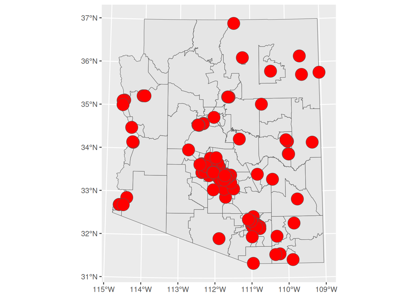
Distance
Often we may want to see how far populations are from certain resources. The st_distance command allows us to do just that.
In the following example we calculate the distance from every census tract population weighted centroid to every hosptial within AZ. This generates a matrix of distances.
read_csv("data/US/COP2020/COP2020_tract.txt") %>%
filter(STATEFP == "04") %>%
st_as_sf(coords = c("LONGITUDE", "LATITUDE"), crs = 4326) %>%
st_distance(AZ_hosp)| 418834.8 [m] | 513413.9 [m] | 394927.7 [m] | 401342.2 [m] | 580851.5 [m] | 237198.5 [m] | 144967.4 [m] | 312153.8 [m] | 407064.0 [m] | 411000.9 [m] | 418508.9 [m] | 415022.4 [m] | 418765.5 [m] | 401926.9 [m] | 419477.3 [m] | 419011.2 [m] | 410801.4 [m] | 415688.1 [m] | 462340.2 [m] | 479213.2 [m] | 414507.0 [m] | 515745.6 [m] | 511192.3 [m] | 513245.8 [m] | 464652.3 [m] | 299981.1 [m] | 510752.5 [m] | 418248.8 [m] | 505678.9 [m] | 420970.6 [m] | 414545.3 [m] | 511192.3 [m] | 416609.9 [m] | 418248.8 [m] | 466325.2 [m] | 512493.3 [m] | 418765.5 [m] | 506313.1 [m] | 418248.8 [m] | 416609.9 [m] | 422789.4 [m] | 414206.8 [m] | 410709.5 [m] | 432473.6 [m] | 520064.2 [m] | 493167.6 [m] | 321776.9 [m] | 134282.591 [m] | 142571.2 [m] | 446391.6 [m] | 390185.8 [m] | 322428.9 [m] | 583224.2 [m] | 340912.5 [m] | 520338.0 [m] | 416255.0 [m] | 595016.7 [m] | 417683.1 [m] | 329530.0 [m] | 612145.0 [m] | 424412.6 [m] | 408594.4 [m] | 289743.3 [m] | 416519.3 [m] | 416952.9 [m] | 410333.6 [m] | 402240.8 [m] | 421187.3 [m] | 422655.2 [m] | 510575.8 [m] | 431874.4 [m] | 415338.0 [m] | 512021.2 [m] | 330364.5 [m] | 514631.2 [m] | 415217.7 [m] | 437196.7 [m] | 120824.18 [m] | 297467.6 [m] | 535802.3 [m] | 500823.0 [m] | 383997.5 [m] | 438936.7 [m] | 497415.3 [m] | 418836.9 [m] | 409309.1 [m] | 418088.5 [m] | 399306.2 [m] | 414984.7 [m] | 399873.8 [m] | 410174.4 [m] | 409270.2 [m] | 411605.2 [m] | 285790.5 [m] | 207238.4 [m] | 506081.8 [m] | 513523.9 [m] | 342156.5 [m] | 630527.1 [m] | 506063.7 [m] | 515536.1 [m] | 429635.8 [m] | 235074.2 [m] | 520620.7 [m] | 394927.7 [m] | 414129.8 [m] | 427831.6 [m] | 399012.4 [m] | 409191.3 [m] | 406292.6 [m] | 630337.0 [m] | 416952.9 [m] | 426473.8 [m] | 119382.28 [m] | 497802.6 [m] | 570913.2 [m] | 415236.0 [m] | 425087.9 [m] | 518777.5 [m] | 420279.0 [m] | 604048.2 [m] | 340848.2 [m] | 73500.537 [m] | 470984.0 [m] | 412865.9 [m] | 413454.5 [m] | 392788.6 [m] | 413137.1 [m] | 341697.1 [m] | 413279.4 [m] | 423761.5 [m] | 414828.6 [m] | 424995.4 [m] | 434088.0 [m] | 418672.9 [m] | 406570.3 [m] | 400647.9 [m] | 429297.9 [m] | 426780.5 [m] | 413498.4 [m] | 236357.9 [m] | 419164.4 [m] | 391066.6 [m] | 428519.3 [m] | 505678.9 [m] | 382301.6 [m] | 419133.9 [m] | 503205.0 [m] | 424843.1 [m] | 415085.8 [m] | 419343.1 [m] | 418529.5 [m] | 545155.3 [m] | 419347.1 [m] | 623743.6 [m] | 459359.3 [m] | 413416.5 [m] |
| 442157.8 [m] | 524284.0 [m] | 418543.8 [m] | 423948.9 [m] | 585561.1 [m] | 269397.1 [m] | 188378.8 [m] | 333760.8 [m] | 432334.1 [m] | 433450.8 [m] | 440203.7 [m] | 441386.5 [m] | 442107.7 [m] | 426685.4 [m] | 442646.6 [m] | 441275.4 [m] | 433302.9 [m] | 441213.3 [m] | 503204.4 [m] | 517404.3 [m] | 455078.6 [m] | 527002.8 [m] | 521601.9 [m] | 524119.3 [m] | 483027.8 [m] | 330919.8 [m] | 521202.6 [m] | 441809.4 [m] | 517218.3 [m] | 441358.9 [m] | 439951.5 [m] | 521601.9 [m] | 439907.0 [m] | 441809.4 [m] | 507210.1 [m] | 522549.7 [m] | 442107.7 [m] | 517823.8 [m] | 441809.4 [m] | 439907.0 [m] | 446152.4 [m] | 434813.9 [m] | 433243.2 [m] | 457741.8 [m] | 530705.7 [m] | 504484.5 [m] | 326473.0 [m] | 116905.672 [m] | 181868.2 [m] | 465793.9 [m] | 398746.0 [m] | 326998.0 [m] | 588748.4 [m] | 373017.3 [m] | 531261.2 [m] | 439796.5 [m] | 597203.6 [m] | 443984.0 [m] | 361276.9 [m] | 621512.0 [m] | 444759.8 [m] | 428336.3 [m] | 295120.2 [m] | 439810.7 [m] | 439817.6 [m] | 450830.6 [m] | 424863.9 [m] | 446330.3 [m] | 443911.8 [m] | 520959.6 [m] | 455552.3 [m] | 441410.1 [m] | 522238.6 [m] | 362064.6 [m] | 525092.4 [m] | 441316.0 [m] | 454635.9 [m] | 119074.53 [m] | 293415.5 [m] | 541438.3 [m] | 502990.0 [m] | 396960.4 [m] | 440393.2 [m] | 534072.7 [m] | 441901.9 [m] | 433241.0 [m] | 441175.8 [m] | 421915.0 [m] | 438915.5 [m] | 422572.2 [m] | 435056.1 [m] | 429662.5 [m] | 436629.5 [m] | 291830.0 [m] | 227426.2 [m] | 517630.0 [m] | 523714.5 [m] | 374491.3 [m] | 662528.0 [m] | 517583.5 [m] | 525028.5 [m] | 454531.4 [m] | 266958.4 [m] | 530025.2 [m] | 418543.8 [m] | 438081.6 [m] | 449113.9 [m] | 422811.4 [m] | 429565.2 [m] | 436473.2 [m] | 662329.1 [m] | 439817.6 [m] | 451212.1 [m] | 144098.59 [m] | 534546.1 [m] | 587439.6 [m] | 438661.8 [m] | 450709.2 [m] | 528970.1 [m] | 440120.2 [m] | 636008.0 [m] | 372959.5 [m] | 73190.757 [m] | 511545.7 [m] | 434334.9 [m] | 438259.8 [m] | 416196.4 [m] | 433653.7 [m] | 373959.9 [m] | 433703.6 [m] | 445789.8 [m] | 437888.4 [m] | 443584.3 [m] | 459372.5 [m] | 441767.4 [m] | 425944.4 [m] | 425448.4 [m] | 454154.7 [m] | 448038.8 [m] | 433230.7 [m] | 268451.7 [m] | 442526.6 [m] | 416556.4 [m] | 449616.1 [m] | 517218.3 [m] | 406733.7 [m] | 439088.2 [m] | 515392.5 [m] | 445132.7 [m] | 440455.8 [m] | 445902.2 [m] | 441840.6 [m] | 555740.3 [m] | 442559.7 [m] | 655380.5 [m] | 480771.0 [m] | 433997.3 [m] |
| 374473.8 [m] | 429418.4 [m] | 352467.7 [m] | 355090.9 [m] | 481961.5 [m] | 240075.2 [m] | 247279.7 [m] | 266714.7 [m] | 370145.0 [m] | 363863.7 [m] | 368538.6 [m] | 381909.9 [m] | 374474.5 [m] | 363319.9 [m] | 374554.8 [m] | 370965.1 [m] | 363849.6 [m] | 379399.9 [m] | 500799.9 [m] | 498919.0 [m] | 452229.4 [m] | 432706.6 [m] | 426063.2 [m] | 429260.9 [m] | 402650.7 [m] | 291501.4 [m] | 425730.9 [m] | 374746.0 [m] | 423505.7 [m] | 366566.1 [m] | 377856.1 [m] | 426063.2 [m] | 372232.9 [m] | 374746.0 [m] | 504835.5 [m] | 426465.1 [m] | 374474.5 [m] | 424056.7 [m] | 374746.0 [m] | 372232.9 [m] | 378436.9 [m] | 360737.2 [m] | 363872.1 [m] | 394660.3 [m] | 435404.2 [m] | 410601.2 [m] | 226480.9 [m] | 5686.274 [m] | 195526.5 [m] | 388069.2 [m] | 302508.2 [m] | 226812.7 [m] | 486042.8 [m] | 334930.2 [m] | 436386.8 [m] | 372752.7 [m] | 490990.8 [m] | 384234.7 [m] | 322617.8 [m] | 523438.0 [m] | 369767.5 [m] | 352474.2 [m] | 197262.5 [m] | 372125.4 [m] | 371051.3 [m] | 447644.8 [m] | 356013.9 [m] | 383292.5 [m] | 371076.7 [m] | 425390.1 [m] | 388338.9 [m] | 381109.3 [m] | 426400.2 [m] | 323193.1 [m] | 429587.1 [m] | 381092.2 [m] | 372992.6 [m] | 41594.13 [m] | 184465.8 [m] | 439221.1 [m] | 397316.3 [m] | 308182.8 [m] | 334549.1 [m] | 507782.8 [m] | 373570.8 [m] | 367440.2 [m] | 372925.4 [m] | 353137.4 [m] | 372911.1 [m] | 353995.5 [m] | 371711.8 [m] | 355254.0 [m] | 373613.4 [m] | 195156.3 [m] | 167447.9 [m] | 423925.8 [m] | 427816.9 [m] | 337143.1 [m] | 615179.9 [m] | 423834.3 [m] | 428079.4 [m] | 390549.9 [m] | 236804.3 [m] | 432888.5 [m] | 352467.7 [m] | 372160.9 [m] | 376178.3 [m] | 357048.5 [m] | 355117.3 [m] | 388791.4 [m] | 614954.1 [m] | 371051.3 [m] | 386919.4 [m] | 120154.44 [m] | 508633.9 [m] | 501482.2 [m] | 371359.9 [m] | 388828.4 [m] | 433009.3 [m] | 364111.0 [m] | 588973.4 [m] | 334898.9 [m] | 60132.588 [m] | 506856.5 [m] | 362318.3 [m] | 374594.0 [m] | 349671.3 [m] | 359403.6 [m] | 336383.3 [m] | 359236.7 [m] | 374754.7 [m] | 369680.0 [m] | 364687.6 [m] | 396282.4 [m] | 373515.1 [m] | 349327.7 [m] | 362243.2 [m] | 390081.6 [m] | 375078.9 [m] | 357189.0 [m] | 238865.6 [m] | 374930.4 [m] | 355587.4 [m] | 376225.6 [m] | 423505.7 [m] | 343289.4 [m] | 363368.4 [m] | 422760.8 [m] | 369996.1 [m] | 378243.5 [m] | 386816.9 [m] | 374136.7 [m] | 460053.8 [m] | 374580.8 [m] | 606903.8 [m] | 407244.1 [m] | 359885.8 [m] |
| 411224.3 [m] | 484801.1 [m] | 388013.6 [m] | 392518.2 [m] | 543509.6 [m] | 249879.8 [m] | 203963.1 [m] | 302232.5 [m] | 403209.3 [m] | 401830.4 [m] | 407926.3 [m] | 413249.6 [m] | 411191.1 [m] | 397124.0 [m] | 411578.4 [m] | 409455.4 [m] | 401726.5 [m] | 412271.1 [m] | 496611.6 [m] | 504673.4 [m] | 447990.4 [m] | 487701.3 [m] | 481906.5 [m] | 484638.3 [m] | 448060.4 [m] | 308804.8 [m] | 481527.2 [m] | 411083.4 [m] | 478080.6 [m] | 408051.8 [m] | 410905.1 [m] | 481906.5 [m] | 408964.5 [m] | 411083.4 [m] | 500652.9 [m] | 482687.9 [m] | 411191.1 [m] | 478670.3 [m] | 411083.4 [m] | 408964.5 [m] | 415229.9 [m] | 401710.3 [m] | 401694.0 [m] | 428458.7 [m] | 491098.6 [m] | 465269.2 [m] | 285019.9 [m] | 73038.156 [m] | 176487.0 [m] | 431630.6 [m] | 358570.5 [m] | 285495.4 [m] | 546961.8 [m] | 351878.2 [m] | 491787.4 [m] | 409066.0 [m] | 554410.4 [m] | 415768.8 [m] | 339804.8 [m] | 581161.2 [m] | 411403.2 [m] | 394614.2 [m] | 254098.7 [m] | 408863.9 [m] | 408507.2 [m] | 443578.7 [m] | 393441.2 [m] | 416998.5 [m] | 411264.4 [m] | 481253.6 [m] | 424849.0 [m] | 412989.1 [m] | 482451.9 [m] | 340524.7 [m] | 485413.1 [m] | 412920.9 [m] | 419153.1 [m] | 77925.82 [m] | 249728.6 [m] | 499755.5 [m] | 460291.6 [m] | 359005.2 [m] | 397597.2 [m] | 518476.8 [m] | 410749.1 [m] | 402893.0 [m] | 410046.1 [m] | 390499.2 [m] | 408531.5 [m] | 391227.4 [m] | 405553.4 [m] | 396423.4 [m] | 407248.3 [m] | 251102.9 [m] | 196417.9 [m] | 478495.7 [m] | 483912.1 [m] | 353634.9 [m] | 639648.8 [m] | 478435.1 [m] | 484905.7 [m] | 424922.6 [m] | 247084.4 [m] | 489852.5 [m] | 388013.6 [m] | 407721.1 [m] | 416458.6 [m] | 392413.4 [m] | 396312.8 [m] | 412440.1 [m] | 639439.6 [m] | 408507.2 [m] | 421478.8 [m] | 121079.19 [m] | 519094.7 [m] | 550920.4 [m] | 407837.8 [m] | 421799.2 [m] | 489156.7 [m] | 406407.4 [m] | 613160.8 [m] | 351829.3 [m] | 38508.305 [m] | 504107.5 [m] | 401910.1 [m] | 408666.6 [m] | 385500.3 [m] | 400487.1 [m] | 353015.2 [m] | 400466.0 [m] | 413751.0 [m] | 406754.9 [m] | 408945.0 [m] | 430095.2 [m] | 410640.3 [m] | 391964.1 [m] | 395933.7 [m] | 424512.6 [m] | 415370.1 [m] | 399474.1 [m] | 248817.4 [m] | 411624.7 [m] | 387746.1 [m] | 416812.1 [m] | 478080.6 [m] | 377013.8 [m] | 405465.4 [m] | 476588.5 [m] | 411730.3 [m] | 411372.4 [m] | 417928.0 [m] | 410898.7 [m] | 516052.6 [m] | 411529.0 [m] | 632069.0 [m] | 448059.8 [m] | 400878.2 [m] |
| 375571.1 [m] | 454554.7 [m] | 352226.4 [m] | 357013.0 [m] | 517079.5 [m] | 213458.0 [m] | 185629.9 [m] | 266685.4 [m] | 367076.2 [m] | 366395.4 [m] | 372733.7 [m] | 376925.1 [m] | 375532.7 [m] | 361087.8 [m] | 375967.3 [m] | 374094.9 [m] | 366276.3 [m] | 376103.3 [m] | 462953.0 [m] | 469183.9 [m] | 414255.2 [m] | 457252.1 [m] | 451906.3 [m] | 454389.7 [m] | 414154.5 [m] | 272085.1 [m] | 451503.5 [m] | 375367.4 [m] | 447454.6 [m] | 373286.0 [m] | 374759.0 [m] | 451906.3 [m] | 373312.7 [m] | 375367.4 [m] | 466999.6 [m] | 452886.9 [m] | 375532.7 [m] | 448061.2 [m] | 375367.4 [m] | 373312.7 [m] | 379575.6 [m] | 366851.1 [m] | 366234.5 [m] | 392374.1 [m] | 460993.8 [m] | 434727.7 [m] | 257715.0 [m] | 69223.198 [m] | 145427.5 [m] | 397285.5 [m] | 329207.6 [m] | 258280.3 [m] | 520015.9 [m] | 315196.5 [m] | 461529.8 [m] | 373350.1 [m] | 529681.0 [m] | 379459.5 [m] | 303107.3 [m] | 551961.2 [m] | 376661.6 [m] | 360032.2 [m] | 226102.4 [m] | 373213.4 [m] | 372972.1 [m] | 409796.0 [m] | 357933.9 [m] | 380919.3 [m] | 376219.5 [m] | 451266.1 [m] | 389134.0 [m] | 376716.8 [m] | 452560.2 [m] | 303823.1 [m] | 455393.4 [m] | 376643.7 [m] | 385539.7 [m] | 52026.30 [m] | 228976.5 [m] | 472644.2 [m] | 435402.3 [m] | 327216.3 [m] | 373051.5 [m] | 482381.6 [m] | 375164.3 [m] | 367063.6 [m] | 374453.6 [m] | 354987.7 [m] | 372715.4 [m] | 355692.9 [m] | 369508.1 [m] | 361620.4 [m] | 371175.3 [m] | 222637.9 [m] | 160536.8 [m] | 447866.1 [m] | 454039.1 [m] | 316971.8 [m] | 602897.2 [m] | 447820.6 [m] | 455429.8 [m] | 388913.1 [m] | 210619.2 [m] | 460439.5 [m] | 352226.4 [m] | 371898.0 [m] | 381419.9 [m] | 356591.6 [m] | 361515.6 [m] | 375700.7 [m] | 602688.1 [m] | 372972.1 [m] | 385498.1 [m] | 84616.82 [m] | 483024.9 [m] | 518028.2 [m] | 372149.2 [m] | 385629.4 [m] | 459295.9 [m] | 371827.8 [m] | 576408.4 [m] | 315148.2 [m] | 4054.704 [m] | 470144.3 [m] | 366770.9 [m] | 372644.7 [m] | 349759.7 [m] | 365654.6 [m] | 316346.2 [m] | 365664.8 [m] | 378472.3 [m] | 371161.6 [m] | 374838.6 [m] | 394010.2 [m] | 375047.3 [m] | 357506.0 [m] | 359885.7 [m] | 388510.9 [m] | 380336.2 [m] | 364911.4 [m] | 212381.4 [m] | 375962.1 [m] | 351537.5 [m] | 381834.6 [m] | 447454.6 [m] | 341003.9 [m] | 370842.8 [m] | 445615.9 [m] | 377009.6 [m] | 375234.6 [m] | 381577.1 [m] | 375247.8 [m] | 486038.4 [m] | 375906.1 [m] | 595324.9 [m] | 413060.6 [m] | 366025.2 [m] |
| 378943.7 [m] | 455596.3 [m] | 355691.1 [m] | 360286.5 [m] | 517005.9 [m] | 218844.0 [m] | 191983.3 [m] | 269977.8 [m] | 370812.4 [m] | 369624.9 [m] | 375816.6 [m] | 380840.0 [m] | 378908.8 [m] | 364742.6 [m] | 379311.5 [m] | 377278.7 [m] | 369515.4 [m] | 379870.1 [m] | 469230.7 [m] | 475017.2 [m] | 420525.0 [m] | 458361.3 [m] | 452867.2 [m] | 455432.0 [m] | 416581.9 [m] | 277040.4 [m] | 452471.9 [m] | 378783.0 [m] | 448620.7 [m] | 376131.0 [m] | 378506.6 [m] | 452867.2 [m] | 376684.1 [m] | 378783.0 [m] | 473277.8 [m] | 453784.1 [m] | 378908.8 [m] | 449221.8 [m] | 378783.0 [m] | 376684.1 [m] | 382949.1 [m] | 369745.5 [m] | 369479.5 [m] | 396069.5 [m] | 461990.6 [m] | 435862.7 [m] | 257770.8 [m] | 63856.791 [m] | 152056.0 [m] | 399918.7 [m] | 329926.1 [m] | 258310.8 [m] | 520083.6 [m] | 320236.9 [m] | 462576.6 [m] | 376765.5 [m] | 529167.0 [m] | 383359.1 [m] | 308115.6 [m] | 552689.7 [m] | 379494.1 [m] | 362779.4 [m] | 226331.3 [m] | 376583.9 [m] | 376266.1 [m] | 416058.1 [m] | 361208.9 [m] | 384610.0 [m] | 379217.6 [m] | 452222.7 [m] | 392549.6 [m] | 380580.1 [m] | 453486.3 [m] | 308821.6 [m] | 456361.4 [m] | 380511.8 [m] | 387831.3 [m] | 50845.01 [m] | 227339.2 [m] | 472746.4 [m] | 434901.8 [m] | 328759.7 [m] | 372438.3 [m] | 487944.9 [m] | 378491.0 [m] | 370559.6 [m] | 377785.4 [m] | 358265.2 [m] | 376201.9 [m] | 358985.3 [m] | 373170.6 [m] | 364483.9 [m] | 374860.6 [m] | 223005.0 [m] | 164053.8 [m] | 449033.5 [m] | 454959.5 [m] | 322047.3 [m] | 607561.0 [m] | 448982.9 [m] | 456224.8 [m] | 392547.2 [m] | 215966.9 [m] | 461215.9 [m] | 355691.1 [m] | 375389.6 [m] | 384415.0 [m] | 360081.5 [m] | 364375.9 [m] | 380290.2 [m] | 607350.4 [m] | 376266.1 [m] | 389109.3 [m] | 90076.99 [m] | 488602.1 [m] | 520034.5 [m] | 375545.7 [m] | 389398.1 [m] | 460213.7 [m] | 374575.4 [m] | 581083.7 [m] | 320189.9 [m] | 6363.175 [m] | 476367.9 [m] | 369822.1 [m] | 376288.3 [m] | 353191.1 [m] | 368534.4 [m] | 321410.8 [m] | 368527.7 [m] | 381606.7 [m] | 374493.7 [m] | 377353.7 [m] | 397706.1 [m] | 378379.4 [m] | 360189.9 [m] | 363550.1 [m] | 392138.7 [m] | 383328.6 [m] | 367649.4 [m] | 217755.2 [m] | 379341.0 [m] | 355340.7 [m] | 384795.5 [m] | 448620.7 [m] | 344636.9 [m] | 373612.4 [m] | 446899.5 [m] | 379831.1 [m] | 378975.0 [m] | 385519.2 [m] | 378618.7 [m] | 487011.1 [m] | 379258.2 [m] | 599930.5 [m] | 416036.4 [m] | 368916.1 [m] |
Often, we may only be interested in the closest facility, and with a little bit more work we can add a column to our population weighted centroid dataset detailing the distance to the closest hospital. First, we will use st_nearest_feature() to get the index position of the closest hospital within our hospital dataset. Then, we use st_distance() to calculate the distance between each population weighted centroid and its closest hospital. Notice that st_distance() has been given the parameter by_element = TRUE, which yields a vector with the distance between the first elements of x and y, the second, etc.
read_csv("data/US/COP2020/COP2020_tract.txt") %>%
filter(STATEFP == "04") %>%
st_as_sf(coords = c("LONGITUDE", "LATITUDE"), crs = 4326) %>%
mutate(nearest = st_nearest_feature(., AZ_hosp)) %>%
mutate(near_distance = st_distance(., AZ_hosp[nearest,], by_element = TRUE)) %>%
select(-nearest)| STATEFP | COUNTYFP | TRACTCE | POPULATION | geometry | near_distance |
|---|---|---|---|---|---|
| 04 | 001 | 942600 | 1549 | POINT (-109.8449 36.76841) | 73500.537 [m] |
| 04 | 001 | 942700 | 4491 | POINT (-109.3544 36.77035) | 73190.757 [m] |
| 04 | 001 | 944000 | 5348 | POINT (-109.088 35.78314) | 5686.274 [m] |
| 04 | 001 | 944100 | 5495 | POINT (-109.2781 36.37803) | 38508.305 [m] |
| 04 | 001 | 944201 | 4021 | POINT (-109.6018 36.17521) | 4054.704 [m] |
Geocoding
You may not always have the latitude and longitude data for some set of point data that you are interested, but you may have addresses. That’s where geocoding comes in. Geocoding is a process that allows us to retrieve coordinates for address data.
tidygeocoder is the most user friendly package for this kind of work. tidygeocoder interfaces with multiple geocoders. Check out the different geocoding options here.
Note
Addresses alone are sufficient information to reidentify individuals. If you are working with sensitivity data DO NOT use a non-compliant geocoder.
library(tidygeocoder)
AZ_hosp %>%
mutate(addr =
str_c(ADDRESS, ", ", CITY, ", AZ ", ZIP)) %>%
slice_head(n = 5) %>%
geocode(addr, method = "osm")Passing 5 addresses to the Nominatim single address geocoderQuery completed in: 5 seconds| OBJECTID | OBJECTID_1 | RUN_DATE | source | BUREAU | FACID | FACILITY_N | LICENSE_NU | LICENSE_EF | LICENSE_EX | MEDICARE_I | MEDICARE_1 | MEDICARE_2 | TELEPHONE | FACILITY_T | TYPE | SUBTYPE | CATEGORY | ICON_CATEG | MEDICARE_T | LICENSE_TY | LICENSE_SU | CAPACITY | ADDRESS | CITY | ZIP | COUNTY | OPERATION_ | X_Is_Publi | HOSPITAL_G | KeyID | ADHSCODE | N_AddressT | N_LocatorT | N_ADDRESS | N_ADDR2 | N_CITY | N_COUNTY | N_FULLADDR | N_LAT | N_LON | N_STATE | N_ZIP | N_ZIP4 | N_BLOCK | RESERVATIO | RESERV_ID | R_METHOD | oPCA | oPCA_ID | P_Method | P_Reliable | SOURCE_VW | CASELOAD | addr | geometry | lat | long |
|---|---|---|---|---|---|---|---|---|---|---|---|---|---|---|---|---|---|---|---|---|---|---|---|---|---|---|---|---|---|---|---|---|---|---|---|---|---|---|---|---|---|---|---|---|---|---|---|---|---|---|---|---|---|---|---|---|---|
| 1 | 2822 | 2024-05-06 | ASPEN | MED | AZTH00002 | BANNER- UNIVERSITY MEDICAL CENTER PHOENIX | NA | NA | NA | 039802 | NA | NA | (602)239-2716 | NA | HOSPITAL | TRANSPLANT | HOSPITAL | HOSPITAL | HOSPITAL - TRANSPLANT HOSPITAL | FEDERAL ONLY | NA | 0 | 1441 N 12TH | PHOENIX | 85006 | MARICOPA | ACTIVE | Yes | NA | AZTH00002 | A | AS0 | CENTRUS-TOMTOM | 1441 N 12TH ST | NA | PHOENIX | MARICOPA COUNTY | 1441 N 12TH ST , PHOENIX, AZ 85006-2837 | 33.46410 | -112.0562 | AZ | 85006 | 2837 | 4.013113e+13 | NA | NA | NA | CENTRAL CITY VILLAGE | 39 | Coordinates | NA | Tableau.vw_licensing_facilities | NA | 1441 N 12TH, PHOENIX, AZ 85006 | POINT (-112.0562 33.46411) | NA | NA |
| 2 | 2823 | 2024-05-06 | ASPEN | MED | AZTH00003 | BANNER UNIVERSITY MEDICAL CTR AT THE AZ HEALTH SC | NA | NA | NA | 039800 | NA | NA | (520)694-0111 | NA | HOSPITAL | TRANSPLANT | HOSPITAL | HOSPITAL | HOSPITAL - TRANSPLANT HOSPITAL | FEDERAL ONLY | NA | 0 | 1501 NORTH CAMPBELL AVENUE | TUCSON | 85724 | PIMA | ACTIVE | Yes | NA | AZTH00003 | A | AS0 | CENTRUS-TOMTOM | 1501 N CAMPBELL AVE | NA | TUCSON | PIMA COUNTY | 1501 N CAMPBELL AVE , TUCSON, AZ 85724-0001 | 32.24080 | -110.9443 | AZ | 85724 | 1 | 4.019002e+13 | NA | NA | NA | TUCSON CENTRAL | 107 | Coordinates | NA | Tableau.vw_licensing_facilities | NA | 1501 NORTH CAMPBELL AVENUE, TUCSON, AZ 85724 | POINT (-110.9443 32.24081) | 32.24123 | -110.9456 |
| 3 | 2824 | 2024-05-06 | ASPEN | MED | AZTH00004 | MAYO CLINIC HOSPITAL | NA | NA | NA | 039801 | NA | NA | (480)342-1900 | NA | HOSPITAL | TRANSPLANT | HOSPITAL | HOSPITAL | HOSPITAL - TRANSPLANT HOSPITAL | FEDERAL ONLY | NA | 0 | 5777 EAST MAYO BOULEVARD | PHOENIX | 85054 | MARICOPA | ACTIVE | Yes | NA | AZTH00004 | A | AS0 | CENTRUS-TOMTOM | 5777 E MAYO BLVD | NA | PHOENIX | MARICOPA COUNTY | 5777 E MAYO BLVD , PHOENIX, AZ 85054-4502 | 33.66316 | -111.9557 | AZ | 85054 | 4502 | 4.013615e+13 | NA | NA | NA | DESERT VIEW VILLAGE | 30 | Coordinates | NA | Tableau.vw_licensing_facilities | NA | 5777 EAST MAYO BOULEVARD, PHOENIX, AZ 85054 | POINT (-111.9557 33.66317) | 33.65883 | -111.9553 |
| 4 | 3774 | 2024-05-06 | ASPEN | MED | BH7347 | VIA LINDA BEHAVIORAL HOSPITAL | SH11520 | 2023-03-01 | 2025-02-28 | 034040 | NA | NA | (480)476-7000 | 12 | HOSPITAL | PSYCHIATRIC | HOSPITAL | HOSPITAL | HOSPITAL - PSYCHIATRIC | HOSPITAL | HOSPITAL - SPECIAL | 120 | 9160 EAST HORSESHOE RD | SCOTTSDALE | 85258 | MARICOPA | ACTIVE | Yes | NA | BH7347 | A | AS0 | CENTRUS-TOMTOM | 9160 E HORSESHOE RD | NA | SCOTTSDALE | MARICOPA COUNTY | 9160 E HORSESHOE RD , SCOTTSDALE, AZ 85258-4666 | 33.56670 | -111.8840 | AZ | 85258 | 4666 | 4.013941e+13 | Salt River Reservation | 3340F | Coordinates | SALT RIVER PIMA-MARICOPA INDIAN COMMUNITY | 62 | Coordinates | NA | Tableau.vw_licensing_facilities | NA | 9160 EAST HORSESHOE RD, SCOTTSDALE, AZ 85258 | POINT (-111.884 33.56671) | 33.56763 | -111.8837 |
| 5 | 4893 | 2024-05-06 | ASPEN | MED | MED0198 | CANYON VISTA MEDICAL CENTER | H7130 | 2020-02-18 | 2024-12-27 | 030043 | NA | NA | (520)263-2220 | 11 | HOSPITAL | SHORT TERM | HOSPITAL | HOSPITAL | HOSPITAL - SHORT TERM | HOSPITAL | HOSPITAL - GENERAL | 100 | 5700 EAST HIGHWAY 90 | SIERRA VISTA | 85635 | COCHISE | ACTIVE | Yes | NA | MED0198 | A | AS0 | CENTRUS-TOMTOM | 5700 E HIGHWAY 90 | NA | SIERRA VISTA | COCHISE COUNTY | 5700 E HIGHWAY 90 , SIERRA VISTA, AZ 85635-9110 | 31.55449 | -110.2319 | AZ | 85635 | 9110 | 4.003002e+13 | NA | NA | NA | SIERRA VISTA | 123 | Coordinates | NA | Tableau.vw_licensing_facilities | NA | 5700 EAST HIGHWAY 90, SIERRA VISTA, AZ 85635 | POINT (-110.2319 31.5545) | NA | NA |
Best Practices
The following are to get you thinking about some best practices when you are working with your own data. Although these remarks may be short, they can be remarkably important to your development as a geospatial analyst.
Map Making
Map making is an art that involves an iterative process of making a map, getting feedback from stakeholders (or even giving yourself feedback), making a map, getting more feedback and so on.
At the very least you should be thinking about
- Audience - who is going to see your map, what information might be relevant to them, how much familiarity does the viewer have with the data
- Medium - how is your map going to be shared, what degree of interaction can the user have with your map, where is the audience going to see your map
- Message - what is the message you hope your audience takes away
Section 508 Compliance
Section 508 refers to a portion of the Rehabilitation Act of 1973 in the United States that mandates that federal agencies ensure that their electronic and information technology is accessible to people with disabilities. Even if you don’t work within a federal agency, Section 508 sets out a good framework for ensuring that our maps are truly accessible to all.
In practice, this can take form as…
- Using a monochromatic color scale (unless appropriate)
- Providing descriptive text or alt text
- If possible, including map, description, and data together
For more information about accessibility guidelines. Check out these Map Accessibility guidelines published by the Minnesota IT Services.
Be Careful With Location Data
Location data alone is sufficient information to reidentify an individual, business, or other entity. If you have been provided with sensitive location data, it is paramount that you maintain the privacy of the data.
This means…
- Not using a non-compliant geocoder - remember you’re sending those addresses to the geocoding service
- Masking data - aggregating data through a spatial join and depicting that data with a symbol map or dot density map will allow you to represent the data without exposing potentially sensitive information
- Removing georeferenced data from PDFs or other georeferenced formats
Provide Metadata
It is a good practice to add the following information to your map:
- Author
- Date
- Data source and year