
Discover indicators
Let’s set our health atlas. For this example we will use the Chicago
Health Atlas. We can do so by calling ha_set() with the
Chicago Health Atlas URL.
ha_set("chicagohealthatlas.org")If we need to check which health atlas we are using, we can use
ha_get().
ha_get()
#> [1] "https://chicagohealthatlas.org/api/v1/"
We can list all the topics (aka indicators) present within Chicago
Health Atlas by using ha_topics(). The most important
column here is the topic_key. An individual
topic_key can be used to identify a topic within subsequent
functions.
topics <- ha_topics(progress = FALSE)
topics
#> # A tibble: 483 × 7
#>    topic_name             topic_key topic_description topic_units topic_keywords
#>    <chr>                  <chr>     <chr>             <chr>       <list>
#>  1 9th grade education r… EDA       Residents 25 or … % of resid… <chr [2]>
#>  2 ACA marketplace enrol… ENR       Number of plan s… plan selec… <chr [5]>
#>  3 Accidents mortality    VRAC      Number of people… count of d… <chr [2]>
#>  4 Accidents mortality r… VRACR     Age-adjusted rat… per 100,00… <chr [2]>
#>  5 Active business licen… CHANVYI   Count of active … licenses p… <chr [1]>
#>  6 Active transportation… ACT       Percent of worke… % of worke… <chr [3]>
#>  7 Adult asthma           HCSATH    Number of adults… count of a… <chr [2]>
#>  8 Adult asthma rate      HCSATHP   Percent of adult… % of adults <chr [2]>
#>  9 Adult binge drinking   HCSBD     Number of adults… count of a… <chr [1]>
#> 10 Adult binge drinking … HCSBDP    Percent of adult… % of adults <chr [1]>
#> # ℹ 473 more rows
#> # ℹ 2 more variables: topic_datasets <list>, topic_subcategories <list>
Note: topics can be derived from multiple datasets
or belong to multiple subcategories or keywords. Therefore, these
columns may be composed of tibbles or vectors. Filtering
topics via these pieces of information is still quite easy using
purrr::map_lgl().
library(dplyr)
library(purrr)

# filter by dataset
topics %>%
  filter(map_lgl(topic_datasets, ~ "healthy-chicago-survey" %in% .x$key))
#> # A tibble: 0 × 7
#> # ℹ 7 variables: topic_name <chr>, topic_key <chr>, topic_description <chr>,
#> #   topic_units <chr>, topic_keywords <list>, topic_datasets <list>,
#> #   topic_subcategories <list>

# filter by subcategory
topics %>%
  filter(map_lgl(topic_subcategories, ~ "diet-exercise" %in% .x$key))
#> # A tibble: 20 × 7
#>    topic_name             topic_key topic_description topic_units topic_keywords
#>    <chr>                  <chr>     <chr>             <chr>       <list>
#>  1 Adult fruit and veget… HCSFV     "Number of adult… count of a… <chr [2]>
#>  2 Adult fruit and veget… HCSFVP    "Percent of adul… % of adults <chr [2]>
#>  3 Adult physical inacti… HCSPA     "Number of adult… count of a… <chr [2]>
#>  4 Adult physical inacti… HCSPAP    "Percent of adul… % of adults <chr [2]>
#>  5 Adult soda consumption HCSS      "Number of adult… count of a… <chr [1]>
#>  6 Adult soda consumptio… HCSSP     "Percent of adul… % of adults <chr [1]>
#>  7 Easy access to fruits… HCSFVA    "Number of adult… count of a… <chr [2]>
#>  8 Easy access to fruits… HCSFVAP   "Percent of adul… % of adults <chr [2]>
#>  9 High School fruit and… YRFV      "Number of Chica… count of s… <chr [2]>
#> 10 High School fruit and… YRFVP     "Percent of Chic… % of stude… <chr [2]>
#> 11 High School physical … YRPA      "Number of Chica… count of s… <chr [0]>
#> 12 High School physical … YRPAP     "Percent of Chic… % of stude… <chr [0]>
#> 13 High School physical … YRPI      "Number of Chica… count of s… <chr [3]>
#> 14 High School physical … YRPIP     "Percent of Chic… % of stude… <chr [3]>
#> 15 High School soda cons… YRSO      "Number of Chica… count of s… <chr [1]>
#> 16 High School soda cons… YRSOP     "Percent of Chic… % of stude… <chr [1]>
#> 17 Middle School physica… YRMPA     "Number of Chica… count of s… <chr [0]>
#> 18 Middle School physica… YRMPAP    "Percent of Chic… % of stude… <chr [0]>
#> 19 Middle School physica… YRMPI     "Number of Chica… count of s… <chr [3]>
#> 20 Middle School physica… YRMPIP    "Percent of Chic… % of stude… <chr [3]>
#> # ℹ 2 more variables: topic_datasets <list>, topic_subcategories <list>

# filter by keyword
topics %>%
  filter(map_lgl(topic_keywords, ~ "activity" %in% .x))
#> # A tibble: 6 × 7
#>   topic_name              topic_key topic_description topic_units topic_keywords
#>   <chr>                   <chr>     <chr>             <chr>       <list>
#> 1 Adult physical inactiv… HCSPA     Number of adults… count of a… <chr [2]>
#> 2 Adult physical inactiv… HCSPAP    Percent of adult… % of adults <chr [2]>
#> 3 High School physical i… YRPI      Number of Chicag… count of s… <chr [3]>
#> 4 High School physical i… YRPIP     Percent of Chica… % of stude… <chr [3]>
#> 5 Middle School physical… YRMPI     Number of Chicag… count of s… <chr [3]>
#> 6 Middle School physical… YRMPIP    Percent of Chica… % of stude… <chr [3]>
#> # ℹ 2 more variables: topic_datasets <list>, topic_subcategories <list>
There may be a specific topic area you are interested in exploring.
You can explore these topic areas using
ha_subcategories().
subcategories <- ha_subcategories()
subcategories
#> # A tibble: 30 × 3
#>    subcategory_name      subcategory_key       category_name
#>    <chr>                 <chr>                 <chr>
#>  1 Access to Care        access-to-care        Clinical Care
#>  2 Quality of Care       quality-of-care       Clinical Care
#>  3 Community Safety      community-safety      Physical Environment
#>  4 Housing & Transit     housing-transit       Physical Environment
#>  5 Pollution             pollution-26          Physical Environment
#>  6 Resource Availability resource-availability Physical Environment
#>  7 Behavioral Health     behavioral-health-2   Morbidity
#>  8 Chronic Disease       chronic-disease-31    Morbidity
#>  9 Infectious Disease    infectious-disease    Morbidity
#> 10 Injury & Violence     injury-violence-1     Morbidity
#> # ℹ 20 more rows
You can use a subcategory_key to subset the list of
topics.
ha_topics("diet-exercise")
#> # A tibble: 20 × 7
#>    topic_name             topic_key topic_description topic_units topic_keywords
#>    <chr>                  <chr>     <chr>             <chr>       <list>
#>  1 Adult fruit and veget… HCSFV     "Number of adult… count of a… <chr [2]>
#>  2 Adult fruit and veget… HCSFVP    "Percent of adul… % of adults <chr [2]>
#>  3 Adult physical inacti… HCSPA     "Number of adult… count of a… <chr [2]>
#>  4 Adult physical inacti… HCSPAP    "Percent of adul… % of adults <chr [2]>
#>  5 Adult soda consumption HCSS      "Number of adult… count of a… <chr [1]>
#>  6 Adult soda consumptio… HCSSP     "Percent of adul… % of adults <chr [1]>
#>  7 Easy access to fruits… HCSFVA    "Number of adult… count of a… <chr [2]>
#>  8 Easy access to fruits… HCSFVAP   "Percent of adul… % of adults <chr [2]>
#>  9 High School fruit and… YRFV      "Number of Chica… count of s… <chr [2]>
#> 10 High School fruit and… YRFVP     "Percent of Chic… % of stude… <chr [2]>
#> 11 High School physical … YRPA      "Number of Chica… count of s… <chr [0]>
#> 12 High School physical … YRPAP     "Percent of Chic… % of stude… <chr [0]>
#> 13 High School physical … YRPI      "Number of Chica… count of s… <chr [3]>
#> 14 High School physical … YRPIP     "Percent of Chic… % of stude… <chr [3]>
#> 15 High School soda cons… YRSO      "Number of Chica… count of s… <chr [1]>
#> 16 High School soda cons… YRSOP     "Percent of Chic… % of stude… <chr [1]>
#> 17 Middle School physica… YRMPA     "Number of Chica… count of s… <chr [0]>
#> 18 Middle School physica… YRMPAP    "Percent of Chic… % of stude… <chr [0]>
#> 19 Middle School physica… YRMPI     "Number of Chica… count of s… <chr [3]>
#> 20 Middle School physica… YRMPIP    "Percent of Chic… % of stude… <chr [3]>
#> # ℹ 2 more variables: topic_datasets <list>, topic_subcategories <list>
Once we have a topic or topics in mind, we can explore what
populations, time periods, and geographic scales that data is available
at by using ha_coverage(). Again, the most important
columns here are the key columns which can be used to specify the data
desired.
coverage <- ha_coverage("HCSFVAP", progress = FALSE)
coverage
#> # A tibble: 187 × 7
#>    topic_key population_key population_name population_grouping period_key
#>    <chr>     <chr>          <chr>           <chr>               <chr>
#>  1 HCSFVAP   ""             Full population ""                  2020-2021
#>  2 HCSFVAP   ""             Full population ""                  2023-2024
#>  3 HCSFVAP   ""             Full population ""                  2021-2022
#>  4 HCSFVAP   ""             Full population ""                  2016-2018
#>  5 HCSFVAP   ""             Full population ""                  2015-2017
#>  6 HCSFVAP   ""             Full population ""                  2022-2023
#>  7 HCSFVAP   ""             Full population ""                  2014-2016
#>  8 HCSFVAP   ""             Full population ""                  2023-2024
#>  9 HCSFVAP   ""             Full population ""                  2024
#> 10 HCSFVAP   ""             Full population ""                  2022-2023
#> # ℹ 177 more rows
#> # ℹ 2 more variables: layer_key <chr>, layer_name <chr>
Import tabular data
Now, we can import our data using ha_data() and
specifying the keys we identified above.
ease_of_access <- ha_data(
  topic_key = "HCSFVAP",
  population_key = "",
  period_key = "2022-2023",
  layer_key = "neighborhood"
)
ease_of_access
#> # A tibble: 77 × 7
#>    geoid      topic_key population_key period_key layer_key  value standardError
#>    <chr>      <chr>     <chr>          <chr>      <chr>      <dbl>         <dbl>
#>  1 1714000-14 HCSFVAP   ""             2022-2023  neighborh…  53.0          6.18
#>  2 1714000-18 HCSFVAP   ""             2022-2023  neighborh…  51.0          9.56
#>  3 1714000-2  HCSFVAP   ""             2022-2023  neighborh…  62.7          5.51
#>  4 1714000-43 HCSFVAP   ""             2022-2023  neighborh…  46.0          6.48
#>  5 1714000-45 HCSFVAP   ""             2022-2023  neighborh…  48.8         10.6
#>  6 1714000-47 HCSFVAP   ""             2022-2023  neighborh…  50.4          8.55
#>  7 1714000-52 HCSFVAP   ""             2022-2023  neighborh…  46.5          7.04
#>  8 1714000-6  HCSFVAP   ""             2022-2023  neighborh…  66.6          2.70
#>  9 1714000-49 HCSFVAP   ""             2022-2023  neighborh…  38.1          7.78
#> 10 1714000-24 HCSFVAP   ""             2022-2023  neighborh…  62.3          4.19
#> # ℹ 67 more rows
We can even specify multiple topics, populations, and periods to get
data for. ha_data() will return a combined table with data
for every combination of topic, population, and period requested. A
warning will be given for every invalid combindation of topic,
population, and period requested.
combinations_of_data <- ha_data(
  topic_key = c("POP", "UMP"),
  population_key = c("", "H"),
  period_key = c("2017-2021", "2018-2022", "invalid"),
  layer_key = "neighborhood"
)
#> Warning: Your API call has errors. No results for topic_key = "POP"
#> population_key = "" period_key = "invalid" layer_key = "neighborhood".
#> Warning: Your API call has errors. No results for topic_key = "UMP"
#> population_key = "" period_key = "invalid" layer_key = "neighborhood".
#> Warning: Your API call has errors. No results for topic_key = "POP"
#> population_key = "H" period_key = "invalid" layer_key = "neighborhood".
#> Warning: Your API call has errors. No results for topic_key = "UMP"
#> population_key = "H" period_key = "invalid" layer_key = "neighborhood".
combinations_of_data
#> # A tibble: 1,278 × 7
#>    geoid      topic_key population_key period_key layer_key  value standardError
#>    <chr>      <chr>     <chr>          <chr>      <chr>      <dbl>         <dbl>
#>  1 1714000-14 UMP       ""             2017-2021  neighborh…  6.67         1.46
#>  2 1714000-18 UMP       ""             2017-2021  neighborh…  5.36         2.10
#>  3 1714000-2  UMP       ""             2017-2021  neighborh…  6.66         1.11
#>  4 1714000-43 UMP       ""             2017-2021  neighborh… 16.4          1.84
#>  5 1714000-45 UMP       ""             2017-2021  neighborh… 13.5          5.24
#>  6 1714000-47 UMP       ""             2017-2021  neighborh… 21.5          8.32
#>  7 1714000-52 UMP       ""             2017-2021  neighborh…  8.02         1.69
#>  8 1714000-6  UMP       ""             2017-2021  neighborh…  4.02         0.621
#>  9 1714000-49 UMP       ""             2017-2021  neighborh… 18.7          2.10
#> 10 1714000-24 UMP       ""             2017-2021  neighborh…  3.50         0.608
#> # ℹ 1,268 more rows
If you want to mix and match topics, populations, years, or layers of
data, I recommend creating a table of all the datasets you want, and
purrr::pmap()-ing over the table.
library(tibble)
library(purrr)

# creating a table of data I want
metadata <- tribble(
  ~topic_key , ~population_key , ~period_key , ~layer_key     ,
  "POP"      , ""              , "2017-2021" , "neighborhood" ,
  "HCSFVAP"  , ""              , "2020-2021" , "neighborhood" ,
  "UMP"      , "H"             , "2017-2021" , "neighborhood" ,
)

metadata %>%
  pmap(ha_data)
#> [[1]]
#> # A tibble: 160 × 7
#>    geoid      topic_key population_key period_key layer_key  value standardError
#>    <chr>      <chr>     <chr>          <chr>      <chr>      <dbl>         <dbl>
#>  1 1714000-14 POP       ""             2017-2021  neighbor…  48823         1880.
#>  2 1714000-18 POP       ""             2017-2021  neighbor…  13785         1016.
#>  3 1714000-2  POP       ""             2017-2021  neighbor…  79911         3188.
#>  4 1714000-43 POP       ""             2017-2021  neighbor…  52735         2187.
#>  5 1714000-45 POP       ""             2017-2021  neighbor…   9645          892.
#>  6 1714000-47 POP       ""             2017-2021  neighbor…   2639          430.
#>  7 1714000-52 POP       ""             2017-2021  neighbor…  24453         1470.
#>  8 1714000-6  POP       ""             2017-2021  neighbor… 102608         2049.
#>  9 1714000-49 POP       ""             2017-2021  neighbor…  39253         1820.
#> 10 1714000-24 POP       ""             2017-2021  neighbor…  86867         1885.
#> # ℹ 150 more rows
#>
#> [[2]]
#> # A tibble: 77 × 7
#>    geoid      topic_key population_key period_key layer_key  value standardError
#>    <chr>      <chr>     <chr>          <chr>      <chr>      <dbl>         <dbl>
#>  1 1714000-14 HCSFVAP   ""             2020-2021  neighborh…  59.6          7.18
#>  2 1714000-18 HCSFVAP   ""             2020-2021  neighborh…  46.3          9.32
#>  3 1714000-2  HCSFVAP   ""             2020-2021  neighborh…  61.8          5.95
#>  4 1714000-43 HCSFVAP   ""             2020-2021  neighborh…  58.5          6.90
#>  5 1714000-45 HCSFVAP   ""             2020-2021  neighborh…  55.7         10.4
#>  6 1714000-47 HCSFVAP   ""             2020-2021  neighborh…  19.0          7.30
#>  7 1714000-52 HCSFVAP   ""             2020-2021  neighborh…  49.0         11.8
#>  8 1714000-6  HCSFVAP   ""             2020-2021  neighborh…  77.5          2.31
#>  9 1714000-49 HCSFVAP   ""             2020-2021  neighborh…  54.9          7.55
#> 10 1714000-24 HCSFVAP   ""             2020-2021  neighborh…  76.1          3.17
#> # ℹ 67 more rows
#>
#> [[3]]
#> # A tibble: 158 × 7
#>    geoid     topic_key population_key period_key layer_key   value standardError
#>    <chr>     <chr>     <chr>          <chr>      <chr>       <dbl>         <dbl>
#>  1 1714000-… UMP       H              2017-2021  neighbor… 6.50e+0          1.59
#>  2 1714000-… UMP       H              2017-2021  neighbor… 3.27e+0          1.83
#>  3 1714000-2 UMP       H              2017-2021  neighbor… 4.56e+0          3.54
#>  4 1714000-… UMP       H              2017-2021  neighbor… 1.77e+1         26.8
#>  5 1714000-… UMP       H              2017-2021  neighbor… 1.48e-1        126.
#>  6 1714000-… UMP       H              2017-2021  neighbor… 5.43e-3         33.0
#>  7 1714000-… UMP       H              2017-2021  neighbor… 7.91e+0          1.68
#>  8 1714000-6 UMP       H              2017-2021  neighbor… 4.38e+0          2.97
#>  9 1714000-… UMP       H              2017-2021  neighbor… 4.71e+1         26.7
#> 10 1714000-… UMP       H              2017-2021  neighbor… 4.13e+0          1.63
#> # ℹ 148 more rows
Import spatial data
We can see all the geographic layers available by using
ha_layers().
layers <- ha_layers()
layers
#> # A tibble: 7 × 3
#>   layer_name      layer_key    layer_url
#>   <chr>           <chr>        <chr>
#> 1 Community areas neighborhood https://media.metop.io/shapes/ancestries/communi…
#> 2 ZIP Codes       zip          https://media.metop.io/shapes/teams/chicago-heal…
#> 3 Census Tracts   tract-2020   https://media.metop.io/shapes/teams/chicago-heal…
#> 4 Chicago         place        https://media.metop.io/shapes/teams/chicago-heal…
#> 5 United States   us           https://media.metop.io/shapes/us.topo.json
#> 6 States          state        https://media.metop.io/shapes/teams/chicago-heal…
#> 7 Counties        county       https://media.metop.io/shapes/teams/chicago-heal…
Since we just downloaded our data at the Community Area level, let’s
import the Community Area geographic layer with
ha_layer().
community_areas <- ha_layer("neighborhood")
community_areas
#> Simple feature collection with 77 features and 6 fields
#> Geometry type: MULTIPOLYGON
#> Dimension:     XY
#> Bounding box:  xmin: -87.94011 ymin: 41.64454 xmax: -87.52419 ymax: 42.02305
#> Geodetic CRS:  WGS 84
#> First 10 features:
#>         geoid    layer_key                         name population state
#> 1   1714000-1 neighborhood    Rogers Park (Chicago, IL)      55454    IL
#> 2  1714000-10 neighborhood   Norwood Park (Chicago, IL)      41069    IL
#> 3  1714000-11 neighborhood Jefferson Park (Chicago, IL)      26201    IL
#> 4  1714000-12 neighborhood    Forest Glen (Chicago, IL)      19579    IL
#> 5  1714000-13 neighborhood     North Park (Chicago, IL)      17522    IL
#> 6  1714000-14 neighborhood    Albany Park (Chicago, IL)      48549    IL
#> 7  1714000-15 neighborhood   Portage Park (Chicago, IL)      63038    IL
#> 8  1714000-16 neighborhood    Irving Park (Chicago, IL)      51911    IL
#> 9  1714000-17 neighborhood        Dunning (Chicago, IL)      43120    IL
#> 10 1714000-18 neighborhood      Montclare (Chicago, IL)      14412    IL
#>             notes                       geometry
#> 1  Far North Side MULTIPOLYGON (((-87.65456 4...
#> 2  Far North Side MULTIPOLYGON (((-87.78002 4...
#> 3  Far North Side MULTIPOLYGON (((-87.75264 4...
#> 4  Far North Side MULTIPOLYGON (((-87.72642 4...
#> 5  Far North Side MULTIPOLYGON (((-87.7069 41...
#> 6  Far North Side MULTIPOLYGON (((-87.70404 4...
#> 7  Northwest Side MULTIPOLYGON (((-87.75264 4...
#> 8  Northwest Side MULTIPOLYGON (((-87.69475 4...
#> 9  Northwest Side MULTIPOLYGON (((-87.77621 4...
#> 10 Northwest Side MULTIPOLYGON (((-87.78942 4...
You can also set geometry = TRUE within your data call
to get the geographic layer’s geometry along with your data.
ease_of_access <- ha_data(
  topic_key = "HCSFVAP",
  population_key = "",
  period_key = "2022-2023",
  layer_key = "neighborhood",
  geometry = TRUE
)
ease_of_access
#> Simple feature collection with 77 features and 7 fields
#> Geometry type: MULTIPOLYGON
#> Dimension:     XY
#> Bounding box:  xmin: -87.94011 ymin: 41.64454 xmax: -87.52419 ymax: 42.02305
#> Geodetic CRS:  WGS 84
#> First 10 features:
#>         geoid topic_key population_key period_key    layer_key    value
#> 1   1714000-1   HCSFVAP                 2022-2023 neighborhood 56.70447
#> 2  1714000-10   HCSFVAP                 2022-2023 neighborhood 61.06724
#> 3  1714000-11   HCSFVAP                 2022-2023 neighborhood 61.46267
#> 4  1714000-12   HCSFVAP                 2022-2023 neighborhood 81.03884
#> 5  1714000-13   HCSFVAP                 2022-2023 neighborhood 54.84689
#> 6  1714000-14   HCSFVAP                 2022-2023 neighborhood 52.98553
#> 7  1714000-15   HCSFVAP                 2022-2023 neighborhood 61.05424
#> 8  1714000-16   HCSFVAP                 2022-2023 neighborhood 61.62744
#> 9  1714000-17   HCSFVAP                 2022-2023 neighborhood 72.73395
#> 10 1714000-18   HCSFVAP                 2022-2023 neighborhood 51.01435
#>    standardError                       geometry
#> 1       4.958576 MULTIPOLYGON (((-87.65456 4...
#> 2       5.929492 MULTIPOLYGON (((-87.78002 4...
#> 3       5.845823 MULTIPOLYGON (((-87.75264 4...
#> 4       4.560229 MULTIPOLYGON (((-87.72642 4...
#> 5      10.003305 MULTIPOLYGON (((-87.7069 41...
#> 6       6.182114 MULTIPOLYGON (((-87.70404 4...
#> 7       5.687155 MULTIPOLYGON (((-87.75264 4...
#> 8       6.953888 MULTIPOLYGON (((-87.69475 4...
#> 9       5.353022 MULTIPOLYGON (((-87.77621 4...
#> 10      9.557330 MULTIPOLYGON (((-87.78942 4...
Let’s map our data!
library(ggplot2)

plot <- ggplot(ease_of_access) +
  geom_sf(aes(fill = value), alpha = 0.7) +
  scale_fill_distiller(palette = "GnBu", direction = 1) +
  labs(
    title = "Easy Access to Fruits and Vegetables within Chicago",
    fill = "Percent of adults who reported\nthat it is very easy for them to\nget fresh fruits and vegetables."
  ) +
  theme_minimal()
plot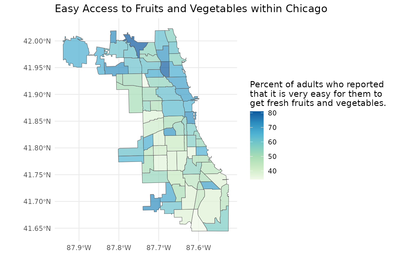
Our map looks pretty good, but perhaps there is a point layer that
may provide more insight into the spatial variation of the ease of
access to fruits and vegetables. We can use
ha_point_layers() to list all the point layers available in
the Chicago Health Atlas.
point_layers <- ha_point_layers()
point_layers
#> # A tibble: 10 × 3
#> point_layer_name point_layer_uuid point_layer_descript…¹
#> <chr> <chr> <chr>
#> 1 Acute Care Hospitals - 2023 67f58fa0-0dfa-4… ""
#> 2 Chicago Public Schools - 2023 5a449804-a2cc-4… ""
#> 3 Federally Qualified Health Centers -… 22f48fd6-ee98-4… ""
#> 4 Federally Qualified Health Centers (… f224b3ce-6d83-4… ""
#> 5 Grocery Stores 7d9caf3c-75e6-4… "All chain grocery st…
#> 6 Hospitals 8768fad7-65a2-4… "https://hifld-geopla…
#> 7 Nursing Homes 379a55c7-e569-4… "https://hifld-geopla…
#> 8 Pharmacies and Drug Stores 93ace519-6ba2-4… "All chain pharmacies…
#> 9 Skilled Nursing Facilities - 2023 93bc497d-3881-4… ""
#> 10 WIC Offices - 2023 7c8e9992-4e25-4… ""
#> # ℹ abbreviated name: ¹point_layer_descriptionGrocery store locations may be an important aspect of the ease of
access to fruits and vegetables. We can import this layer by providing
the point_layer_uuid to ha_point_layer().
grocery_stores <- ha_point_layer("7d9caf3c-75e6-4382-8c97-069696a3efbf")Now that we have imported our grocery stores, let’s layer them on top of our map.
plot +
  geom_sf(data = grocery_stores, size = 0.5)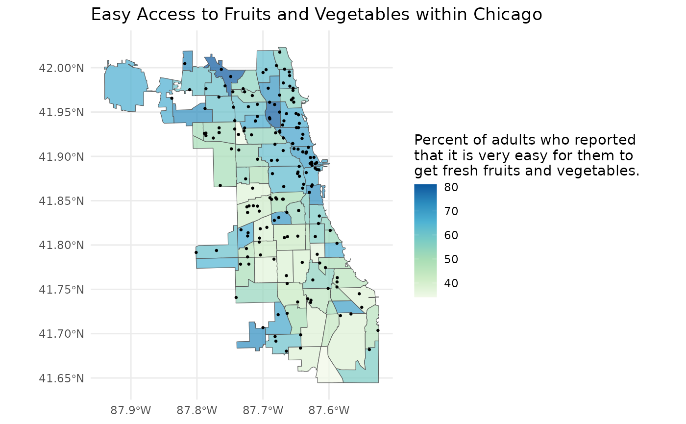
As expected, it seems that the areas with more grocery stores tend to have a higher percent of adults who report that it is very easy to get fresh fruits and vegetables.
This is a typical use case for the healthatlas in which
we explored every function that healthatlas has to offer.
Now it’s time for you to explore!