Discover indicators
Let’s set our health atlas. For this example we will use the Chicago
Health Atlas. We can do so by calling ha_set() with the
Chicago Health Atlas URL.
ha_set("chicagohealthatlas.org")If we need to check which health atlas we are using, we can use
ha_get().
ha_get()
#> [1] "https://chicagohealthatlas.org/api/v1/"
We can list all the topics (aka indicators) present within Chicago
Health Atlas by using ha_topics(). The most important
column here is the topic_key. An individual
topic_key can be used to identify a topic within subsequent
functions.
topics <- ha_topics(progress = FALSE)
#> Error in get(paste0(generic, ".", class), envir = get_method_env()) :
#>   object 'type_sum.accel' not found
topics
#> # A tibble: 409 × 7
#>    topic_name           topic_key topic_description topic_units subcategory_name
#>    <chr>                <chr>     <chr>             <chr>       <chr>
#>  1 9th grade education… EDA       Residents 25 or … % of resid… Education
#>  2 ACA marketplace enr… ENR       Number of plan s… plan selec… Access to Care
#>  3 Accidents mortality  VRAC      Number of people… count of d… Injury & Violen…
#>  4 Accidents mortality… VRACR     Age-adjusted rat… per 100,00… Injury & Violen…
#>  5 Active business lic… CHANVYI   Count of active … licenses p… Income
#>  6 Adult asthma         HCSATH    Number of adults… count of a… Chronic Disease
#>  7 Adult asthma rate    HCSATHP   Percent of adult… % of adults Chronic Disease
#>  8 Adult binge drinking HCSBD     Number of adults… count of a… Alcohol & Drug …
#>  9 Adult binge drinkin… HCSBDP    Percent of adult… % of adults Alcohol & Drug …
#> 10 Adult diabetes       HCSDIA    Number of adults… count of a… Chronic Disease
#> # ℹ 399 more rows
#> # ℹ 2 more variables: subcategory_key <chr>, category_name <chr>
There may be a specific topic area you are interested in exploring.
You can explore these topic areas using
ha_subcategories().
subcategories <- ha_subcategories()
subcategories
#> # A tibble: 30 × 3
#>    subcategory_name      subcategory_key       category_name
#>    <chr>                 <chr>                 <chr>
#>  1 Access to Care        access-to-care        Clinical Care
#>  2 Quality of Care       quality-of-care       Clinical Care
#>  3 Community Safety      community-safety-1    Physical Environment
#>  4 Housing & Transit     housing-transit       Physical Environment
#>  5 Pollution             pollution             Physical Environment
#>  6 Resource Availability resource-availability Physical Environment
#>  7 Behavioral Health     behavioral-health     Morbidity
#>  8 Chronic Disease       chronic-disease-1     Morbidity
#>  9 Infectious Disease    infectious-disease-1  Morbidity
#> 10 Injury & Violence     injury-violence-1     Morbidity
#> # ℹ 20 more rows
You can use a subcategory_key to subset the list of
topics.
ha_topics("diet-exercise")
#> # A tibble: 20 × 7
#>    topic_name           topic_key topic_description topic_units subcategory_name
#>    <chr>                <chr>     <chr>             <chr>       <chr>
#>  1 Adult fruit and veg… HCSFV     "Number of adult… count of a… Diet & Exercise
#>  2 Adult fruit and veg… HCSFVP    "Percent of adul… % of adults Diet & Exercise
#>  3 Adult physical inac… HCSPA     "Number of adult… count of a… Diet & Exercise
#>  4 Adult physical inac… HCSPAP    "Percent of adul… % of adults Diet & Exercise
#>  5 Adult soda consumpt… HCSS      "Number of adult… count of a… Diet & Exercise
#>  6 Adult soda consumpt… HCSSP     "Percent of adul… % of adults Diet & Exercise
#>  7 Easy access to frui… HCSFVA    "Number of adult… count of a… Diet & Exercise
#>  8 Easy access to frui… HCSFVAP   "Percent of adul… % of adults Diet & Exercise
#>  9 High School fruit a… YRFV      "Number of Chica… count of s… Diet & Exercise
#> 10 High School fruit a… YRFVP     "Percent of Chic… % of stude… Diet & Exercise
#> 11 High School physica… YRPA      "Number of Chica… count of s… Diet & Exercise
#> 12 High School physica… YRPAP     "Percent of Chic… % of stude… Diet & Exercise
#> 13 High School physica… YRPI      "Number of Chica… count of s… Diet & Exercise
#> 14 High School physica… YRPIP     "Percent of Chic… % of stude… Diet & Exercise
#> 15 High School soda co… YRSO      "Number of Chica… count of s… Diet & Exercise
#> 16 High School soda co… YRSOP     "Percent of Chic… % of stude… Diet & Exercise
#> 17 Middle School physi… YRMPA     "Number of Chica… count of s… Diet & Exercise
#> 18 Middle School physi… YRMPAP    "Percent of Chic… % of stude… Diet & Exercise
#> 19 Middle School physi… YRMPI     "Number of Chica… count of s… Diet & Exercise
#> 20 Middle School physi… YRMPIP    "Percent of Chic… % of stude… Diet & Exercise
#> # ℹ 2 more variables: subcategory_key <chr>, category_name <chr>
Once we have a topic or topics in mind, we can explore what
populations, time periods, and geographic scales that data is available
at by using ha_coverage(). Again, the most important
columns here are the key columns which can be used to specify the data
desired.
coverage <- ha_coverage("HCSFVAP", progress = FALSE)
coverage
#> # A tibble: 166 × 7
#>    topic_key population_key population_name population_grouping period_key
#>    <chr>     <chr>          <chr>           <chr>               <chr>
#>  1 HCSFVAP   ""             Full population ""                  2020-2021
#>  2 HCSFVAP   ""             Full population ""                  2016-2018
#>  3 HCSFVAP   ""             Full population ""                  2015-2017
#>  4 HCSFVAP   ""             Full population ""                  2014-2016
#>  5 HCSFVAP   ""             Full population ""                  2022-2023
#>  6 HCSFVAP   ""             Full population ""                  2021-2022
#>  7 HCSFVAP   ""             Full population ""                  2022-2023
#>  8 HCSFVAP   ""             Full population ""                  2023
#>  9 HCSFVAP   ""             Full population ""                  2021-2022
#> 10 HCSFVAP   ""             Full population ""                  2022
#> # ℹ 156 more rows
#> # ℹ 2 more variables: layer_key <chr>, layer_name <chr>
Import tabular data
Now, we can import our data using ha_data() and
specifying the keys we identified above.
ease_of_access <- ha_data(
  topic_key = "HCSFVAP",
  population_key = "",
  period_key = "2022-2023",
  layer_key = "neighborhood"
)
ease_of_access
#> # A tibble: 77 × 7
#>    geoid      topic_key population_key period_key layer_key  value standardError
#>    <chr>      <chr>     <chr>          <chr>      <chr>      <dbl>         <dbl>
#>  1 1714000-35 HCSFVAP   ""             2022-2023  neighborh…  57.9          6.86
#>  2 1714000-36 HCSFVAP   ""             2022-2023  neighborh…  54.7          6.25
#>  3 1714000-37 HCSFVAP   ""             2022-2023  neighborh…  45.5          7.45
#>  4 1714000-38 HCSFVAP   ""             2022-2023  neighborh…  56.9          5.86
#>  5 1714000-39 HCSFVAP   ""             2022-2023  neighborh…  52.4         10.5
#>  6 1714000-4  HCSFVAP   ""             2022-2023  neighborh…  71.7          5.49
#>  7 1714000-40 HCSFVAP   ""             2022-2023  neighborh…  36.8          6.73
#>  8 1714000-41 HCSFVAP   ""             2022-2023  neighborh…  65.9          7.52
#>  9 1714000-42 HCSFVAP   ""             2022-2023  neighborh…  48.4          8.27
#> 10 1714000-1  HCSFVAP   ""             2022-2023  neighborh…  56.7          4.96
#> # ℹ 67 more rows
We can even specify multiple topics, populations, and periods to get
data for. ha_data() will return a combined table with data
for every combination of topic, population, and period requested. A
warning will be given for every invalid combindation of topic,
population, and period requested.
combinations_of_data <- ha_data(
  topic_key = c("POP", "UMP"),
  population_key = c("", "H"),
  period_key = c("2017-2021", "2018-2022", "invalid"),
  layer_key = "neighborhood"
)
#> Warning: Your API call has errors. No results for topic_key = "POP"
#> population_key = "" period_key = "invalid" layer_key = "neighborhood".
#> Warning: Your API call has errors. No results for topic_key = "UMP"
#> population_key = "" period_key = "invalid" layer_key = "neighborhood".
#> Warning: Your API call has errors. No results for topic_key = "POP"
#> population_key = "H" period_key = "invalid" layer_key = "neighborhood".
#> Warning: Your API call has errors. No results for topic_key = "UMP"
#> population_key = "H" period_key = "invalid" layer_key = "neighborhood".
combinations_of_data
#> # A tibble: 616 × 7
#>    geoid      topic_key population_key period_key layer_key  value standardError
#>    <chr>      <chr>     <chr>          <chr>      <chr>      <dbl>         <dbl>
#>  1 1714000-35 POP       ""             2017-2021  neighbor… 21276.            NA
#>  2 1714000-36 POP       ""             2017-2021  neighbor…  7417.            NA
#>  3 1714000-37 POP       ""             2017-2021  neighbor…  2280.            NA
#>  4 1714000-38 POP       ""             2017-2021  neighbor… 24397.            NA
#>  5 1714000-39 POP       ""             2017-2021  neighbor… 18503.            NA
#>  6 1714000-4  POP       ""             2017-2021  neighbor… 42252.            NA
#>  7 1714000-40 POP       ""             2017-2021  neighbor… 11608.            NA
#>  8 1714000-41 POP       ""             2017-2021  neighbor… 28802.            NA
#>  9 1714000-42 POP       ""             2017-2021  neighbor… 24362.            NA
#> 10 1714000-1  POP       ""             2017-2021  neighbor… 55627.            NA
#> # ℹ 606 more rows
If you want to mix and match topics, populations, years, or layers of
data, I recommend creating a table of all the datasets you want, and
purrr::pmap()-ing over the table.
library(tibble)
library(purrr)

# creating a table of data I want
metadata <- tribble(
  ~ topic_key, ~ population_key, ~ period_key, ~ layer_key,
  "POP",       "",               "2017-2021",  "neighborhood",
  "HCSFVAP",   "",               "2020-2021",  "neighborhood",
  "UMP",       "H",              "2017-2021",  "neighborhood",
)

metadata %>%
  pmap(ha_data)
#> [[1]]
#> # A tibble: 77 × 7
#>    geoid      topic_key population_key period_key layer_key  value standardError
#>    <chr>      <chr>     <chr>          <chr>      <chr>      <dbl> <lgl>
#>  1 1714000-35 POP       ""             2017-2021  neighbor… 21276. NA
#>  2 1714000-36 POP       ""             2017-2021  neighbor…  7417. NA
#>  3 1714000-37 POP       ""             2017-2021  neighbor…  2280. NA
#>  4 1714000-38 POP       ""             2017-2021  neighbor… 24397. NA
#>  5 1714000-39 POP       ""             2017-2021  neighbor… 18503. NA
#>  6 1714000-4  POP       ""             2017-2021  neighbor… 42252. NA
#>  7 1714000-40 POP       ""             2017-2021  neighbor… 11608. NA
#>  8 1714000-41 POP       ""             2017-2021  neighbor… 28802. NA
#>  9 1714000-42 POP       ""             2017-2021  neighbor… 24362. NA
#> 10 1714000-1  POP       ""             2017-2021  neighbor… 55627. NA
#> # ℹ 67 more rows
#>
#> [[2]]
#> # A tibble: 77 × 7
#>    geoid      topic_key population_key period_key layer_key  value standardError
#>    <chr>      <chr>     <chr>          <chr>      <chr>      <dbl>         <dbl>
#>  1 1714000-35 HCSFVAP   ""             2020-2021  neighborh…  52.0          9.18
#>  2 1714000-36 HCSFVAP   ""             2020-2021  neighborh…  63.8          9.34
#>  3 1714000-37 HCSFVAP   ""             2020-2021  neighborh…  33.2          9.78
#>  4 1714000-38 HCSFVAP   ""             2020-2021  neighborh…  47.4          7.36
#>  5 1714000-39 HCSFVAP   ""             2020-2021  neighborh…  61.3          7.22
#>  6 1714000-4  HCSFVAP   ""             2020-2021  neighborh…  77.4          5.22
#>  7 1714000-40 HCSFVAP   ""             2020-2021  neighborh…  46.2          8.67
#>  8 1714000-41 HCSFVAP   ""             2020-2021  neighborh…  76.3          5.30
#>  9 1714000-42 HCSFVAP   ""             2020-2021  neighborh…  56.4          7.77
#> 10 1714000-1  HCSFVAP   ""             2020-2021  neighborh…  58.0          4.98
#> # ℹ 67 more rows
#>
#> [[3]]
#> # A tibble: 77 × 7
#>    geoid     topic_key population_key period_key layer_key   value standardError
#>    <chr>     <chr>     <chr>          <chr>      <chr>       <dbl>         <dbl>
#>  1 1714000-… UMP       H              2017-2021  neighbor… 20.2            22.8
#>  2 1714000-… UMP       H              2017-2021  neighbor…  0.0239         48.0
#>  3 1714000-… UMP       H              2017-2021  neighbor…  6.60           21.8
#>  4 1714000-… UMP       H              2017-2021  neighbor…  9.47           30.5
#>  5 1714000-… UMP       H              2017-2021  neighbor… 12.2            28.4
#>  6 1714000-4 UMP       H              2017-2021  neighbor…  8.13            3.35
#>  7 1714000-… UMP       H              2017-2021  neighbor… 29.8            52.9
#>  8 1714000-… UMP       H              2017-2021  neighbor…  6.42           10.5
#>  9 1714000-… UMP       H              2017-2021  neighbor…  3.37           37.6
#> 10 1714000-1 UMP       H              2017-2021  neighbor…  5.19            4.38
#> # ℹ 67 more rows
Import spatial data
We can see all the geographic layers available by using
ha_layers().
layers <- ha_layers()
layers
#> # A tibble: 4 × 4
#>   layer_name      layer_key    layer_description                       layer_url
#>   <chr>           <chr>        <chr>                                   <chr>
#> 1 Community areas neighborhood The city of Chicago is divided into 77… https://…
#> 2 ZIP Codes       zip          The ZIP code is a basic unit of geogra… https://…
#> 3 Census Tracts   tract-2020   Census tracts are small geographies de… https://…
#> 4 Chicago         place        Cities, towns, villages, and boroughs,… https://…
Since we just downloaded our data at the Community Area level, let’s
import the Community Area geographic layer with
ha_layer().
community_areas <- ha_layer("neighborhood")
community_areas
#> Simple feature collection with 77 features and 6 fields
#> Geometry type: MULTIPOLYGON
#> Dimension:     XY
#> Bounding box:  xmin: -87.94011 ymin: 41.64454 xmax: -87.52419 ymax: 42.02305
#> Geodetic CRS:  WGS 84
#> First 10 features:
#>         geoid    layer_key                         name population state
#> 1   1714000-1 neighborhood    Rogers Park (Chicago, IL)      55454    IL
#> 2  1714000-10 neighborhood   Norwood Park (Chicago, IL)      41069    IL
#> 3  1714000-11 neighborhood Jefferson Park (Chicago, IL)      26201    IL
#> 4  1714000-12 neighborhood    Forest Glen (Chicago, IL)      19579    IL
#> 5  1714000-13 neighborhood     North Park (Chicago, IL)      17522    IL
#> 6  1714000-14 neighborhood    Albany Park (Chicago, IL)      48549    IL
#> 7  1714000-15 neighborhood   Portage Park (Chicago, IL)      63038    IL
#> 8  1714000-16 neighborhood    Irving Park (Chicago, IL)      51911    IL
#> 9  1714000-17 neighborhood        Dunning (Chicago, IL)      43120    IL
#> 10 1714000-18 neighborhood      Montclare (Chicago, IL)      14412    IL
#>             notes                       geometry
#> 1  Far North Side MULTIPOLYGON (((-87.65456 4...
#> 2  Far North Side MULTIPOLYGON (((-87.78002 4...
#> 3  Far North Side MULTIPOLYGON (((-87.75264 4...
#> 4  Far North Side MULTIPOLYGON (((-87.72642 4...
#> 5  Far North Side MULTIPOLYGON (((-87.7069 41...
#> 6  Far North Side MULTIPOLYGON (((-87.70404 4...
#> 7  Northwest Side MULTIPOLYGON (((-87.75264 4...
#> 8  Northwest Side MULTIPOLYGON (((-87.69475 4...
#> 9  Northwest Side MULTIPOLYGON (((-87.77621 4...
#> 10 Northwest Side MULTIPOLYGON (((-87.78942 4...
You can also set geometry = TRUE within your data call
to get the geographic layer’s geometry along with your data.
ease_of_access <- ha_data(
  topic_key = "HCSFVAP",
  population_key = "",
  period_key = "2022-2023",
  layer_key = "neighborhood",
  geometry = TRUE
)
ease_of_access
#> Simple feature collection with 77 features and 7 fields
#> Geometry type: MULTIPOLYGON
#> Dimension:     XY
#> Bounding box:  xmin: -87.94011 ymin: 41.64454 xmax: -87.52419 ymax: 42.02305
#> Geodetic CRS:  WGS 84
#> First 10 features:
#>         geoid topic_key population_key period_key    layer_key    value
#> 1   1714000-1   HCSFVAP                 2022-2023 neighborhood 56.70447
#> 2  1714000-10   HCSFVAP                 2022-2023 neighborhood 61.06724
#> 3  1714000-11   HCSFVAP                 2022-2023 neighborhood 61.46267
#> 4  1714000-12   HCSFVAP                 2022-2023 neighborhood 81.03884
#> 5  1714000-13   HCSFVAP                 2022-2023 neighborhood 54.84689
#> 6  1714000-14   HCSFVAP                 2022-2023 neighborhood 52.98553
#> 7  1714000-15   HCSFVAP                 2022-2023 neighborhood 61.05424
#> 8  1714000-16   HCSFVAP                 2022-2023 neighborhood 61.62744
#> 9  1714000-17   HCSFVAP                 2022-2023 neighborhood 72.73395
#> 10 1714000-18   HCSFVAP                 2022-2023 neighborhood 51.01435
#>    standardError                       geometry
#> 1       4.958576 MULTIPOLYGON (((-87.65456 4...
#> 2       5.929492 MULTIPOLYGON (((-87.78002 4...
#> 3       5.845823 MULTIPOLYGON (((-87.75264 4...
#> 4       4.560229 MULTIPOLYGON (((-87.72642 4...
#> 5      10.003305 MULTIPOLYGON (((-87.7069 41...
#> 6       6.182114 MULTIPOLYGON (((-87.70404 4...
#> 7       5.687155 MULTIPOLYGON (((-87.75264 4...
#> 8       6.953888 MULTIPOLYGON (((-87.69475 4...
#> 9       5.353022 MULTIPOLYGON (((-87.77621 4...
#> 10      9.557330 MULTIPOLYGON (((-87.78942 4...
Let’s map our data!
library(ggplot2)

plot <- ggplot(ease_of_access) +
  geom_sf(aes(fill = value), alpha = 0.7) +
  scale_fill_distiller(palette = "GnBu", direction = 1) +
  labs(
    title = "Easy Access to Fruits and Vegetables within Chicago",
    fill = "Percent of adults who reported\nthat it is very easy for them to\nget fresh fruits and vegetables."
  ) +
  theme_minimal()
plot
Our map looks pretty good, but perhaps there is a point layer that
may provide more insight into the spatial variation of the ease of
access to fruits and vegetables. We can use
ha_point_layers() to list all the point layers available in
the Chicago Health Atlas.
point_layers <- ha_point_layers()
point_layers
#> # A tibble: 10 × 3
#> point_layer_name point_layer_uuid point_layer_descript…¹
#> <chr> <chr> <chr>
#> 1 Acute Care Hospitals - 2023 67f58fa0-0dfa-4… ""
#> 2 Chicago Public Schools - 2023 5a449804-a2cc-4… ""
#> 3 Federally Qualified Health Centers -… 22f48fd6-ee98-4… ""
#> 4 Federally Qualified Health Centers (… f224b3ce-6d83-4… ""
#> 5 Grocery Stores 7d9caf3c-75e6-4… "All chain grocery st…
#> 6 Hospitals 8768fad7-65a2-4… "https://hifld-geopla…
#> 7 Nursing Homes 379a55c7-e569-4… "https://hifld-geopla…
#> 8 Pharmacies and Drug Stores 93ace519-6ba2-4… "All chain pharmacies…
#> 9 Skilled Nursing Facilities - 2023 93bc497d-3881-4… ""
#> 10 WIC Offices - 2023 7c8e9992-4e25-4… ""
#> # ℹ abbreviated name: ¹point_layer_descriptionGrocery store locations may be an important aspect of the ease of
access to fruits and vegetables. We can import this layer by providing
the point_layer_uuid to ha_point_layer().
grocery_stores <- ha_point_layer("7d9caf3c-75e6-4382-8c97-069696a3efbf")Now that we have imported our grocery stores, let’s layer them on top of our map.
plot +
  geom_sf(data = grocery_stores, size = 0.5)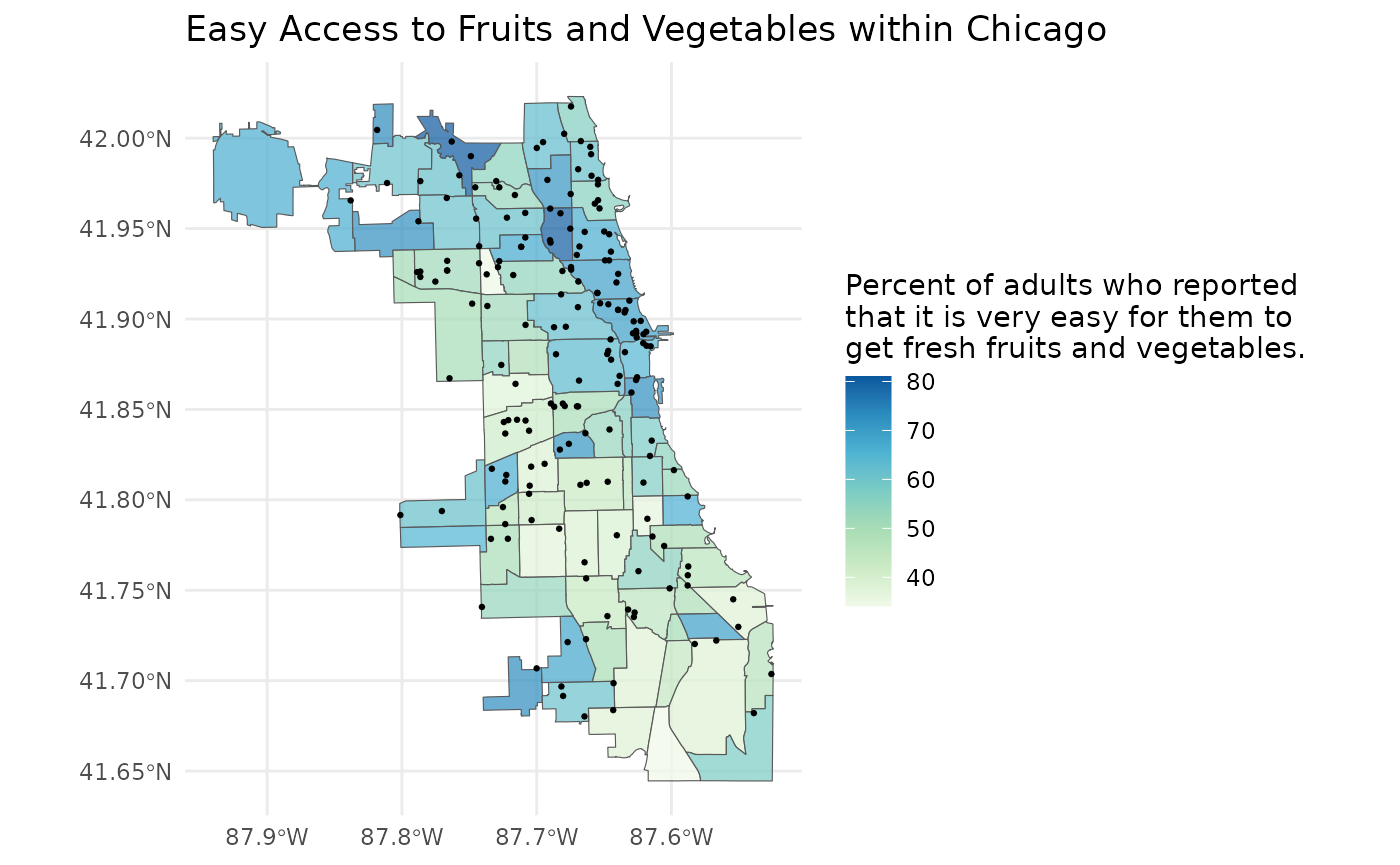
As expected, it seems that the areas with more grocery stores tend to have a higher percent of adults who report that it is very easy to get fresh fruits and vegetables.
This is a typical use case for the healthatlas in which
we explored every function that healthatlas has to offer.
Now it’s time for you to explore!